Space-based gravitational wave signal detection and extraction with deep neural network

ABSTRACT Space-based gravitational wave (GW) detectors will be able to observe signals from sources that are otherwise nearly impossible from current ground-based detection. Consequently,

the well established signal detection method, matched filtering, will require a complex template bank, leading to a computational cost that is too expensive in practice. Here, we develop a

high-accuracy GW signal detection and extraction method for all space-based GW sources. As a proof of concept, we show that a science-driven and uniform multi-stage self-attention-based deep

neural network can identify synthetic signals that are submerged in Gaussian noise. Our method exhibits a detection rate exceeding 99% in identifying signals from various sources, with the

signal-to-noise ratio at 50, at a false alarm rate of 1%. while obtaining at least 95% similarity compared with target signals. We further demonstrate the interpretability and strong

generalization behavior for several extended scenarios. SIMILAR CONTENT BEING VIEWED BY OTHERS CONCEPTS AND STATUS OF CHINESE SPACE GRAVITATIONAL WAVE DETECTION PROJECTS Article 15 September

2021 FIRST FEASIBILITY DEMONSTRATION OF GNSS-SEISMOLOGY FOR ANTHROPOGENIC EARTHQUAKES DETECTION Article Open access 27 November 2023 HARDWARE-ACCELERATED INFERENCE FOR REAL-TIME

GRAVITATIONAL-WAVE ASTRONOMY Article 12 May 2022 INTRODUCTION The first direct detection of GWs coming from coalescing binary black holes (BBHs) was made by the LIGO/Virgo Collaboration1,

which verifies Einstein’s General Relativity. As detectors become more sensitive, more and more GW events are discovered, enabling a new era of multi-messenger astronomy. A total of 93

events have been reported in the three observations2. GWs have become a new probe allowing cross-validation with a variety of fundamental physical theories3,4,5,6. Ground-based GW detectors

such as LIGO, Virgo, and KAGRA cannot detect GWs at frequencies lower than 10Hz due to seismic noise7, therefore space-based detectors are being developed. Laser Interferometer Space Antenna

(LISA) will be launched around 20348, and Taiji9 and TianQin10 are also in progress. LISA is expected to observe a variety of GW sources11, including Galactic binaries (GB), massive black

hole binaries (MBHB), and extreme-mass-ratio-inspirals (EMRI). The most common GB sources are binary white dwarf (BWD) systems, which will populate the whole frequency band of the LISA

detector. Massive black holes (MBH) exist in most galactic centers, and the MBHs merge along with the galaxies, which happens regularly in the Universe12. The EMRI system is formed when the

MBH captures compact objects (CO) surrounding them. Unlike stars, COs can avoid tidal disruption and approach the central MBH, radiating a significant amount of energy in GWs at low

frequencies. Beyond these resolvable sources, a huge number of unresolvable events will sum up incoherently, forming a stochastic GW background (SGWB). The detection of those GWs in the LISA

mission enables us to gain a better understanding of black holes and galaxies13. GW data processing is complicated due to the overwhelming noise, which is non-Gaussian, sometimes

non-stationary14,15, and containing sudden temporary glitches14,15,16. Earlier GW detection methods are divided into two categories: _a_) theoretical template-based algorithms like matched

filtering, _b_) template-independent algorithms. In principle, the most accurate results can be achieved by using a matched filtering algorithm to detect signals buried in Gaussian

noise17,18,19. This is currently the most widely used algorithm for the detection of GWs. The additional complexity of space-based detection over ground-based detection can be attributed to

the different types of sources. The optimal template for matched filtering would have to include all the GW source parameters in the data. However, this is not practical because of the high

parameter space dimension to be explored. Moreover, the typical duration of the compact binary coalescence signal detected by LISA is longer than that detected by ground-based detectors,

resulting in an even larger computational effort for the matched filtering algorithm. For ground-based detection, a series of template-independent signal extraction and detection algorithms

have been developed, such as CWb20, and BayesWave21, both based on the wavelet transformation. Torres et al.22 proposes a total-variation-based method, and a novel approach based on the

Hilbert-Huang transform was recently developed23. The advantage of these algorithms is that they are not limited by theoretical template banks and can extract the signal from noisy data, or,

in other words, reconstruct the signal waveform. The disadvantage of these algorithms is that they are only available for burst signals, which are not suitable for space-based GW signals.

Deep learning has already been successful in various GW data analyses, such as signal detection24,25,26,27,28,29,30, parameter estimation31, 32, glitch classification33,34,35, noise

reduction15, 16, and signal extraction36,37,38,39. Several deep neural network techniques have been used in signal extraction, including dictionary learning36, WaveNet37, denoising

autoencoder38, and LSTM39. Most of these existing methods for detection24, 26,27,28 are designed for ground-based GWs, and for space-based signal30, and40 only achieve single source

detection of EMRI and MBHB signals, respectively. The transformer-based model’s initial application to GW waveform forecasting is presented by Khan et al.41. However, there is no unified

treatment for all sources of the space-based GW signal detection and extraction method. In this article, we develop a uniform deep learning-based model for space-based GW signal detection

and extraction for the four main GW sources of LISA. Our model is based on a self-attention sequence-to-sequence architecture that performs well when dealing with time series data. We have

integrated long-term and short-term feature extraction blocks in our model to catch the dependency of the GW signal in high-dimensional latent space. To our knowledge, this is the first

study to achieve high-accuracy detection and high-precision extraction for all main potential GW signals from space-based detection. The model’s intermediate results can be interpreted as

the encoded signal waveform, revealing a strong correlation between what needs to be learned and what has been learned by the neural network. In our test results analysis, we obtained

average overlaps (see eq. (14)) of 95% of our test samples being >0.95. It takes <10−2 s to perform extraction and detection, which is a factor of roughly 105 improvement over

traditional approaches that often require several hours. Finally, our method can also achieve considerable extraction effects for some signals generated by other models that are not in the

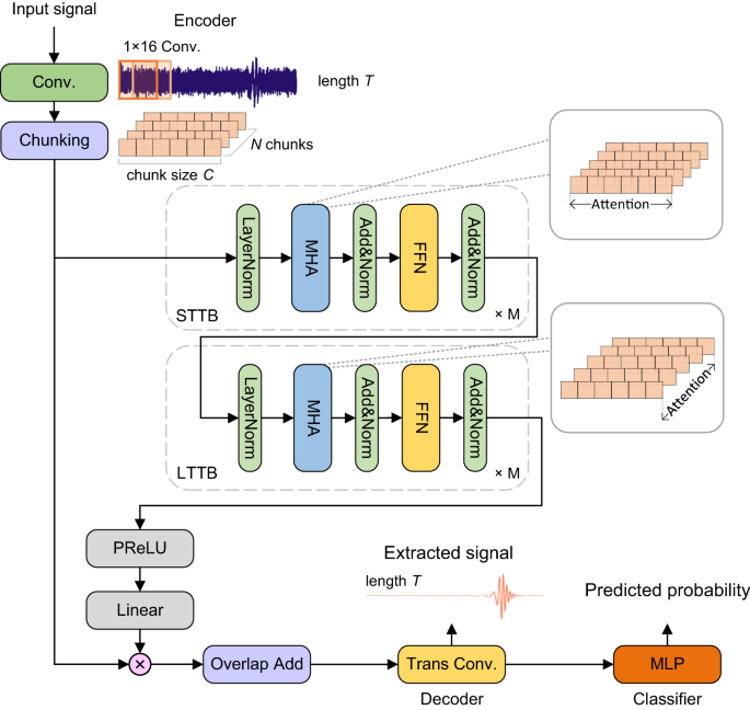
training dataset, demonstrating the strong generalization ability of the model. RESULTS DEEP NEURAL NETWORK We extend the mask-based prediction method for speech enhancement in Conv-TasNet42

with a self-attention-based network for our task. As shown in Fig. 1, the network consists of four processing stages: encoder, extraction net, decoder, and classifier. First, the encoder

maps the signal from the detector to a high-dimensional representation and splits it into short chunks. This encoded representation is used to estimate a mask network for signal extraction.

The extraction network produces a mask matrix with Transformer blocks catching both short-term and long-term dependency from chunks. The decoder uses a transposed convolution layer for the

element-wise multiplying of the mask matrix and an encoded representation to reconstruct the extracted signal. Finally, the extracted signal is sent to a multi-layer linear perception

classifier for detection. The classifier gives the predicted probability that the input data contains a true GW signal. GENERATE SPACE-BASED GWS DATASET Due to the large differences in

signals of GWs from different sources, we generate training and testing datasets for each source. We choose a universal sampling rate of 0.1 Hz for all datasets. All the data samples in the

datasets have 16,000 sampling points, hence the duration of each sample is 160,000 s or 44.4 h. The parameter space of signal generation is sampled with a uniform grid. The range of the

parameters used to generate the GW signals are listed in the Tables 1–3. Then, the parameters on each grid point are used to generate the corresponding GW signals. For noise generation, we

use the noise power spectral density (PSD) of LISA43 to simulate Gaussian noise. It should be noted that in this study, galactic confusion noise has not been taken into consideration. To

simulate the different signal-to-noise ratio (SNR) levels in signal extraction, we set the SNR equal to 50, 40, and 30 following the eq. (12). The SGWB data is directly generated by the PSD

given by eq. (4), in which the parameter _α_ characterizes the amplitude of the SGWB signal. We set _α_ equal to −11.35, −11.55, and −11.75 to generate the signal in the test datasets. To

train the model for the GW detection task, we generate that half of the samples contain signals and half are pure noise. Figure 2 shows some sample cases for our generated data. Specific

details for each dataset will be presented in Methods. INTERPRETABILITY OF THE NETWORK To better understand what information the self-attention-based neural network learned, we explored the

corresponding relationship between the attention mechanism and the embedded input signal. We calculate the attention maps of various layers of the network. The attention map presents the

average output of attention heads in each layer, between each pair of tokens. The output of each attention head is a weighted sum of the embedded tokens of signal, which will be defined in

detail in the Methods. The core of our network is the extraction net, consisting of several STTBs (Short-Time Transformer Block) and LTTBs (Long-Time Transformer Block) stacked together.

Both LTTB and STTB contain multi-head attention layers, which enable our model to have universal learning capability for different GW sources. In STTB, attention is only calculated between

tokens in the same chunk, which indicates that all tokens exchange information within the corresponding chunk. The attention map of STTBs is a diagonal line consisting of squares in chunk

size, implying STTBs are only interested in local structures. And the top panel of each sub-figure in Fig. 3 shows the attention maps between all embedded tokens in LTTB. We can see that for

different GW sources, the model weights show different patterns. We sum each column of the attention map to obtain the attention received by each token, which is called attention weights

(middle panel). As seen for the EMRI, MBHB, and BWD models, the attention weights and the signal after a sliding average follow the same pattern. We also applied the Augmented Dickey-Fuller

(ADF) test to the summed attention map matrix, which is a 1 × 1999 vector, for both the BWD and SGWB models, owing to the stationary nature of the signals in the data. These results were

-6.84 and -15.33, respectively, indicating that the attention maps are also stationary. This means that our LTTB can learn the global dependency of the data. The above experiments show that

our self-attention-based model has the ability to learn both local and global structures for different physical scenarios. GW SIGNAL EXTRACTION The most straightforward test is to use our

model to extract a piece of data with Gaussian noise and see whether it is able to extract the signal. In Fig. 4 we show some examples of the signal extraction effect of our model for

different types of GW signals. Three subplots a,b, and c show the signal extraction effect of our model for EMRI, MBHB, and BWD signals, and the overlap between the model output and the

template is calculated. The overlap shows a very good signal extraction effect. Since SGWB does not have a specific waveform, we do not do this test here for the corresponding model. The

most straightforward test is to use our model to extract a piece of data with Gaussian noise and see whether it is able to extract the signal. In Fig. 4 we show some examples of the signal

extraction effect of our model for different types of GW signals. Three subplots a,b, and c show the signal extraction effect of our model for EMRI, MBHB, and BWD signals, and the overlap

between the model output and the template is calculated. The overlap shows a very good signal extraction effect. Since SGWB does not have a specific waveform, we do not do this test here for

the corresponding model. Then, we perform some statistical tests on the model. We generate the test data in the same way as we generate the training dataset. We use a coarser grid and

create test datasets of 10,000 samples containing signals with SNR equal to 30, 40, and 50 respectively for each type of GW. In the left column of Fig. 4, the signal extraction effect of the

three models for each of the three types of GWs is depicted. The showcase is selected according to the 15 percent quantile of the testing overlap of each GW source. In the right column, it

can be seen that for the case of SNR = 50, the signal extraction effect is performed with great accuracy for MBHB signals, and the overlap is higher than 0.99 for all test samples. The

overlap for the BWD signal is >0.97 for 95% of the test samples. Although it is slightly less effective in extracting the EMRI signal due to its complexity, 92% of samples have overlap

>0.95. GW SIGNAL DETECTION The signals extracted by the neural network are used to build up four new datasets to test the ability of our model to detect GW signals. These four test

datasets each included 10,000 samples containing signals and 10,000 samples containing pure noise. Here we utilize the detection rate, another term for true positive rate (TPR), to measure

the probability of correctly identifying signals. For each signal type and an SNR of (30, 40, 50) and a false alarm rate at 1%, the detection rates are (98.20%, 99.70%, 99.71%) for EMRI,

(99.99%, 100%, 100%) for MBHB, (99.37%, 99.97%, 99.98%) for BWD, respectively. For SGWB signals with _α_ of (−11.75, −11.55, −11.35) and a false alarm rate at 1%, the detection rates are

(95.05%, 99.97%, 100%), respectively. To quantify the performance of our model in detection tasks, we use the receiver operating characteristic (ROC) curve as shown in Fig. 5. In ROC

analysis, the true positive rate (TPR) and the false positive rate (FPR) are plotted as the probability threshold for classifying a candidate as positive (i.e., signal) is altered. The area

under the ROC curve (AUC) has been used to evaluate the classifier’s performance, which is a single scalar value between 0 and 1. In general, the higher the AUC, the better the classifier.

We calculate AUC using Scikit-Learn library44. For all 4 signal types, the AUC are all close to 1, which indicates a fairly high sensitivity for classification (signal detection). TEST ON

LDC2A In the subsequent subsection, we provide an empirical assessment of our model employing the LDC2a dataset. As depicted in Fig. 6, the model proficiently extracts all 15 signals, with

an overlap exceeding 0.9 for each, and notably, 13 of these signals exhibit an overlap above 0.96. Concurrently, the model demonstrates a detection probability equal to 1. The signal #2 has

a lower overlap because it is totally buried in the confusion noise. When compared with MFCNN40, our approach not only ensures the detection of all 15 signals but also generates denoised

waveforms with an overlap >0.9, underlining its efficacy and precision. On the other hand, to draw a comparison with the conventional Markov chain Monte Carlo method45, we conducted the

test using the LDC2a dataset. Detailed results can be found in Supplementary Notes I and Supplementary Table 1. MODEL GENERALIZATION BEHAVIOR Next, we evaluate the generalization ability of

the model. Results are shown in Fig. 7. The parameter space of our EMRI training dataset is only 4-dimensional with a fixed initial semi-latus rectum _p_0 = 20_M_. Figure 7a shows the result

of testing our model using a signal with _p_0 = 30_M_, which indicates a strong generalization capability beyond the training parameter space. The training dataset of MBHB only contains GW

signals from spin-aligned MBHB systems with quasi-circular orbits, without considering the case of orbital eccentricity. Here we generate a GW signal with initial orbital eccentricity _e_0 =

 0.5 using the SEOBNRE model46. In Fig. 7b, we can see the extracted effect, which demonstrates that our model has good generalizability. To test the generalization ability of the BWD model,

our test signal is generated using an evolving BWD system that considers mass transfer, tidal forces, and gravitational radiation effects47. The extracted result is shown in Fig. 7c. The

output detection statistics labeled as detection probabilities of these three test signals are all equal to 1. The final test case is the SGWB model, here we consider broken power law

signals following eq. (5) with parameters _α_ = − 11.18, _n__t_1 = 2/3, _n__t_2 = − 1/3, and _f__T_ = 0.002. This spectral shape might arise from the combination of two physically distinct

sources. The classification test obtained AUC = 0.99997. Then we evaluate our models’ generalization ability to weaker signals. For EMRI, MBHB, and BWD models, we test them using data with

lower SNR, for the SGWB model, we use test data with smaller amplitude. The histogram of overlap between extracted signal and the template is shown in Fig. 4, at the same time the ROC curve

of signal detection results is shown in Fig. 5. Throughout this series of tests, we have demonstrated the generalizability of our models in a wide variety of scenarios. From an astrophysical

perspective, first, LISA will observe MBHBs with very high SNR, typically bigger than 100, out to very high redshift11. Then for EMRI signals, due to its physical complexity, the detection

SNR threshold is ~ 3011. Next, for the LISA verification binaries almost half of them reach a SNR≥3048. Finally, the upper limit of the SGWB is Ω_G__W_(25Hz) ≤ 3.4 × 10−9 for the case of

_n__t_ = 2/3, corresponding to _α_ = − 11.7449. In summary, the generalization ability of the model shows the potential of our model to be applied in practical situations. DISCUSSION With

the results presented above, we show the efficacy of our Transformer-based deep neural network for space-based GW signal extraction and detection of multiple sources. Our method is reusable

for either simulated or future observational data and gives an almost real-time analysis with low computational cost. Detailed results about the speed of our model can be found in

Supplementary Notes II and Supplementary Tables 2–3. One potential limitation of our method is generalization behavior. We show the generalization performance for multiple signals outside

the training dataset, those cases are still simpler than realistic astrophysical conditions. For example, the time delay interferometry technique is normally required to suppress the laser

frequency noise in the space-based GW data analysis, which introduces further complexity in the detector response to the GW signal. Therefore, from a deep learning perspective, the patterns

in the time domain might be different and a re-training of our neural network is required. In this paper, we present a pioneering proof-of-principle study that utilizes DNNs for the

efficient detection and extraction of space-based gravitational wave signals. It’s essential to clarify that our neural network model is not aimed at replace conventional matched filtering

techniques. Instead, it seeks to offer an efficient way of processing the potentially large amount of data from space-based detectors, thereby facilitating more automated and real-time

gravitational wave data analysis. Our model has demonstrated promising results in analyzing MBHB signals, even in datasets with lower signal-to-noise ratios than LDC datasets. Nonetheless,

our approach still faces limitations when addressing long-lasting signals, such as EMRIs and BWDs, which accumulate signal-to-noise ratios over time spans on the order of years. Given the

current computational resources, analyzing these signals in a singular pass poses a considerable challenge Despite the challenges faced, this research stands as a stepping stone in the

domain of GW data analysis. By laying the foundation for future endeavors, we are aiming at the continual development and optimization of deep learning techniques in this field. As

computational resources and technology advance, our model holds the potential for adaptation and evolution to effectively tackle these challenges. METHODS GW SOURCES IN SPACE-BASED DETECTION

As mentioned in the Introduction, space-based GW detectors are being developed to detect GW signals at frequencies of [10−4, 0.1]Hz. The main GW sources in this frequency band are EMRI,

MBHB, BWD, and SGWB. Next, we will describe the details of the signals that come from each GW source. EMRI The MBHs in the centers of galaxies are typically surrounded by clusters of stars.

These stars eventually evolved into COs, which will be black holes, neutron stars, or white dwarfs. Some of those COs can get captured onto orbits bound to the central MBH and then gradually

inspiral into the MBH via emission of GWs. Typically the ratio of the mass of the CO that is falling into the MBH to the mass of the MBH is ~ 10−5, so these events are called EMRIs. EMRI

signal waveforms are characterized by the complex time domain strain _h_(_t_), in the source frame _h_(_t_) is given by50: $$h(t)=\frac{\mu

}{{d}_{L}}\mathop{\sum}\limits_{lmkn}{A}_{lmkn}(t){S}_{lmkn}(t,\theta ){e}^{im\phi }{e}^{-i{\Phi }_{mkn}(t)},$$ (1) where _μ_ is the mass of the small black hole, _t_ is the time of arrival

of the GW, _θ_ is the source-frame polar angle, _ϕ_ is the source-frame azimuthal angle, _d__L_ is the luminosity distance, and {l; m; k; n} are the indices describing harmonic modes. The

indices l, m, k, and n label the orbital angular momentum, azimuthal, polar, and radial modes, respectively. Φ_m__k__n_ = _m_Φ_φ_ + _k_Φ_θ_ + _n_Φ_r_ is the summation of phases for each

mode. _A__l__m__k__n_ is the amplitude of GW. _S__l__m__k__n_(_t_, _θ_) is spin-weighted spheroidal harmonic function. In the detector frame, the EMRI signal waveform is determined by 17

parameters: \(\{M,\mu ,a,{\overrightarrow{a}}_{2},{p}_{0},{e}_{0},{x}_{I,0},{d}_{L},{\theta }_{S},{\phi }_{S},{\theta }_{K},{\phi }_{K},{\Phi }_{\varphi ,0},{\Phi }_{\theta ,0},{\Phi

}_{r,0}\}\). _M_ is the mass of the MBH, _a_ is the dimensionless spin of the MBH, _θ__S_, and _ϕ__S_ are the polar and azimuthal sky location angles. _θ__K_ and _ϕ__K_ are the azimuthal and

polar angles describing the orientation of the spin angular momentum vector of the MBH. \({\overrightarrow{a}}_{2}\) is the spin vector of the CO, which doesn’t considered in the waveform

model. _p_ is semi-latus rectum, _e_ is eccentricity, _I_ is orbit’s inclination angle from the equatorial plane, and \({x}_{I}\equiv \cos I\). MBHB Most galaxies appear to host black holes

at their centers. Galaxies and MBHBs coevolved during the evolution of the Universe. So the observation of GWs from the MBHB system can improve our understanding of important astronomical

phenomena such as the formation of the MBH and the merging of galaxies11. In this paper we just consider the GW from spin-aligned MBHB system, which characterized by

\(\{{M}_{tot},q,{s}_{1}^{z},{s}_{2}^{z}\}\), where _M__t__o__t_ = _m_1 + _m_2, _m_1 and _m_2 are the mass of two black holes respectively. _q_ = _m_2/_m_1 (_m_1 > _m_2) is the mass ratio.

\({s}_{1}^{z}\) and \({s}_{2}^{z}\) are spin parameters of two black holes, and _z_ represent the direction of orbital angular momentum. BWD The Milky Way contains a large population of

compact binaries, most of which are BWD with a period of ~ 1 h. This is right in the LISA’s sensitive frequency band. The signal of BWD in the source frame is quite simple: $${h}_{+}(t)=

{{{{{{{\mathcal{A}}}}}}}}(1+{\cos }^{2}\iota )\cos \Phi (t),\\ {h}_{\times }(t)= 2{{{{{{{\mathcal{A}}}}}}}}\sin \iota \sin \Phi (t),\\ \Phi (t)= {\phi }_{0}+2\pi ft+\pi \dot{f}{t}^{2}.$$ (2)

\({{{{{{{\mathcal{A}}}}}}}}\) is the overall amplitude, _ϕ_0 is the initial phase at the start of the observation, ι is the inclination of the BWD orbit to the line of sight from the origin

of the Solar System Barycentric (SSB) frame. The intrinsic parameter is the frequency of the signal _f_ and its derivative \(\dot{f}\). Frequency evolves slowly and some binaries will be

chirping to higher frequency due to the decay of the orbit through the emission of GWs, but other binaries will be moving to lower frequency as a result of mass transfer between the binary

components driving an increase in the orbital separation11. SGWB There are many resolvable sources, but there is also a large number of events that cannot be resolved individually, resulting

in SGWB. Astrophysical background components are guaranteed in the LISA band, originating from unresolved Galactic Binaries (GB) and stellar-originated black hole mergers. SGWBs that are

Gaussian, isotropic, and stationary can be fully described by their spectrum51: $${\Omega }_{GW}(f)=\frac{f}{{\rho }_{c}}\frac{{{{{{{{\rm{d}}}}}}}}\,{\rho }_{GW}}{{{{{{{{\rm{d}}}}}}}}\,f},$$

(3) where _ρ__G__W_ is the energy density of gravitational radiation contained in the frequency range _f_ to _f_ + _d__f_, \({\rho }_{c}=\frac{3{H}_{0}^{2}{c}^{2}}{8\pi G}\) is the critical

density of the universe, where _c_ is the speed of light, and _G_ is Newton’s constant, _H_0 = 67.9km s−1 Mpc−1 is the Hubble constant. We intend to follow the simplified assumption that

the signal can be well described by a power law, defined as amplitude and slope, as most studies have done previously. Then the signal is described by52: $${h}^{2}{\Omega

}_{GW}(f)=1{0}^{\alpha }{\left(\frac{f}{{f}_{* }}\right)}^{{n}_{t}},$$ (4) where _h_ is dimensionless Hubble constant, _f_* is pivot frequency, _α_ characterize its amplitude at _f_* and

_n__t_ is the slope of spectrum. Another formalism used to test our model’s generalization ability is broken power law which is defined: $${h}^{2}{\Omega }_{GW}(f)=1{0}^{\alpha

}\left[H({f}_{T}-f){\left(\frac{f}{{f}_{* }}\right)}^{{n}_{t1}}+H(f-{f}_{T}){\left(\frac{{f}_{T}}{{f}_{* }}\right)}^{{n}_{t1}}{\left(\frac{f}{{f}_{T}}\right)}^{{n}_{t2}}\right],$$ (5) where

_n__t_1 and _n__t_2 are the slopes of two spectrum segments, _H_(_f_) is Heaviside step function. DATA CURATION First, we simulate the noise data from the LISA sensitivity curve:

$${S}_{n}(f)=\frac{1}{{L}^{2}{{{{{{{\mathcal{R}}}}}}}}(f)}\left({P}_{{{{{{{{\rm{OMS}}}}}}}}}+2(1+{\cos }^{2}(f/{f}_{* }))\frac{{P}_{{{{{{{{\rm{acc}}}}}}}}}}{{(2\pi f)}^{4}}\right),$$ (6)

where $${P}_{{{{{{{{\rm{OMS}}}}}}}}}={(1.5\times 1{0}^{-11}\,{{{{{{{\rm{m}}}}}}}})}^{2}\left(1+{\left(\frac{2\,{{{{{{{\rm{mHz}}}}}}}}}{f}\right)}^{4}\right)\,{{{{{{{{\rm{Hz}}}}}}}}}^{-1}$$

(7) and $${P}_{{{{{{{{\rm{acc}}}}}}}}}={(3\times

1{0}^{-15}\,{{{{{{{\rm{m}}}}}}}})}^{2}\left(1+{\left(\frac{0.4\,{{{{{{{\rm{mHz}}}}}}}}}{f}\right)}^{2}\right)\left(1+{\left(\frac{f}{8\,{{{{{{{\rm{mHz}}}}}}}}}\right)}^{4}\right)\,{{{{{{{{\rm{Hz}}}}}}}}}^{-1}$$

(8) are the optical metrology noise and acceleration noise respectively. _L_ = 2.5 × 109 m, _f_* = 19.09 mHz, \({{{{{{{\mathcal{R}}}}}}}}(f)\) is the transfer function. The full expression

for \({{{{{{{\mathcal{R}}}}}}}}(f)\) used here is computed numerically43. Next we specify the generation of each dataset. We use the augmented analytic kludge (AAK)50, 53, 54 model to

generate the EMRI signal. It is because the AAK model combines the accuracy of the numerical kludge (NK) model and the computational speed of the analytic kludge (AK) model quite well. Note

that the parameter ι in the AAK model is a orbital parameter: \(\cos \iota ={L}_{z}/\sqrt{{L}_{z}^{2}+Q}\), where _Q_ is Carter constant, _L__z_ is _z_ component of the specific angular

momentum. For simplicity, we just consider a small parameter space to generate the training data. Detailed parameters range is shown in Table 1, and the lower bound of _a_ and _e_0 is

limited by the FastEMRIWaveform toolkit we used55. For MBHB signal generation, we used SEOBNRv4_opt, which is a version of the SEOBNRv4 code56 with significant optimizations. It could

produce signals for a high spin, high mass ratio MBHB system. We adopted the log-uniform distribution for the parameter _M__t__o__t_ from Katz et al.57. Detailed parameters range is shown in

Table 2. For the BWD dataset, we generate the signal directly using eq. (2). We follow the parameter setting of the LISA Data Challenge (LDC) 1-4 dataset58, but we focus only on the

intrinsic parameters _f_ and \(\dot{f}\), see Table 3 for details. Upon generating the signal, we project it onto the LISA detector. For this work, being a proof-of-concept, we did not

incorporate the time delay interferometry (TDI) technique. Instead, we employed the long-wavelength approximation, as described below:

$$\begin{array}{rcl}{h}_{I,II}(t)&=&\frac{\sqrt{3}}{2}\left({h}_{+}(t){F}_{I,II}^{+}({\theta }_{S},{\phi }_{S},{\psi }_{S})\right.\\ &&+\left.{h}_{\times

}(t){F}_{I,II}^{\times }({\theta }_{S},{\phi }_{S},{\psi }_{S})\right),\end{array}$$ (9) where \({F}_{I,II}^{+}\) and \({F}_{I,II}^{\times }\) are the antenna pattern functions:

$$\begin{array}{l}{F}_{I}^{+}({\theta }_{S},{\phi }_{S},{\psi }_{S})=\frac{1}{2}(1+{\cos }^{2}{\theta }_{S})(\cos 2{\phi }_{S}\cos 2{\psi }_{S}-\cos {\theta }_{S}\sin 2{\phi }_{S}\sin 2{\psi

}_{S}),\\ {F}_{I}^{\times }({\theta }_{S},{\phi }_{S},{\psi }_{S})=\frac{1}{2}(1+{\cos }^{2}{\theta }_{S})(\cos 2{\phi }_{S}\sin 2{\psi }_{S}+\cos {\theta }_{S}\sin 2{\phi }_{S}\cos 2{\psi

}_{S}),\end{array}$$ (10) and $$\begin{array}{l}{F}_{II}^{+}({\theta }_{S},{\phi }_{S},{\psi }_{S})={F}_{I}^{+}({\theta }_{S},{\phi }_{S},{\psi }_{S}-\pi /4),\\ {F}_{II}^{\times }({\theta

}_{S},{\phi }_{S},{\psi }_{S})={F}_{I}^{\times }({\theta }_{S},{\phi }_{S},{\psi }_{S}-\pi /4),\end{array}$$ (11) where _ψ__S_ is the polarization angle. Furthermore, this antenna pattern

function varies with time as a result of the motion of the LISA detector. In this paper, we set the sky position and the polarization angle equal to zero for simplicity. Because of the

length of our data, the Doppler shift effects could be ignored. For those 3 datasets, we inject the signal to the noise with specific optimal SNR as: $${{{{{{{\rm{SNR}}}}}}}}={\left(s|

s\right)}^{1/2},$$ (12) where _s_ represent the signal template, the inner product (_h_∣_s_) is: $$(h| s)=2\int\nolimits_{{f}_{\min }}^{{f}_{\max }}\frac{{\tilde{h}}^{*

}(f)\tilde{s}(f)+\tilde{h}(f){\tilde{s}}^{* }(f)}{{S}_{n}(f)}\,df,$$ (13) where \({f}_{\min }=3\times 1{0}^{-5}{{{{{{{\rm{Hz}}}}}}}}\) and \({f}_{\max }=0.05{{{{{{{\rm{Hz}}}}}}}}\).

\(\tilde{h}(f)\) and \(\tilde{s}(f)\) are frequency domain signals and the superscript * means complex conjugate, _S__n_(_f_) is the noise PSD. Here following the setting of the LDC dataset,

we set the SNR of the training data to 50. Then the data was whitened and normalized to [−1,1]. During the whitening procedure, we applied the Tukey window with _α_ = 1/8. This inner

product can also be used to measure how well the output of our model matches the signal waveform template, we calculate the overlap between them, which is defined as:

$${{{{{{{\mathcal{O}}}}}}}}(h,s)=\left(\hat{h}| \hat{s}\right)$$ (14) with $$\hat{h}=h{\left(h| h\right)}^{-1/2},$$ (15) where _h_ represent the model output and _s_ represent the template.

The SGWB dataset is generated in a very different way than several other datasets, We just need to simulate SGWB data based on its PSD which is defined by: $${S}_{h}(f)=\frac{3{H}_{0}}{4{\pi

}^{2}}\frac{{\Omega }_{GW}(f)}{{f}^{3}}.$$ (16) We choose _n__t_ = 2/3_α_ = − 11.35 and _f_* = 10−3Hz (see eq. (4)) according to LDC configuration52, which represent SGWB formed by compact

binary coalescences. We could generate the SGWB signal by _S__h_(_f_) directly. We then combine the signal and noise and perform the whitening and normalization operations as described

above. Lastly, we present the pure signals with noise PSD and SGWB PSD in the Fourier domain and the data generated to train our model in Fig. 2. TRANSFORMER Transformer59 is a kind of deep

neural network (DNN) proposed for machine translation, and it soon achieved superior performance in various tasks in natural language processing60 and computer vision61. Based entirely on

attention, Transformer has a great ability to capture both long-range and short-range dependency in sequence data. In this section, we introduce the key structures of a general Transformer.

SELF-ATTENTION Self-Attention can be described as a function with an input vector Query and an output vector pair Key-Value. The Key-Value pair is a weighted sum, which returns the

information of the Query with the corresponding Key. In the Transformer network block, all query vectors and key-values pairs have the same dimension _d_. Given a sequence of queries \(Q\in

{{\mathbb{R}}}^{l\times d}\) with length _l_, keys \(K\in {{\mathbb{R}}}^{l\times d}\) and values \(V\in {{\mathbb{R}}}^{l\times d}\), the Transformer compute scaled dot-product attention

as: $${{{{{{{\rm{Attention}}}}}}}}(Q,K,V)={{{{{{{\rm{softmax}}}}}}}}\left(\frac{Q{K}^{T}}{\sqrt{d}}\right)V.$$ (17) MULTI-HEAD ATTENTION Instead of applying a single attention function with

_d__m__o__d__e__l_-dimensional queries, keys, and values. The Transformer uses multi-head attention to combine information from different linear projections of original queries, keys, and

values. If the Transformer has _H_ heads, the sequence of attention output _h__e__a__d__i_ is:

$$hea{d}_{i}={{{{{{{\rm{Attention}}}}}}}}({Q}_{i},{K}_{i},{V}_{i})={{{{{{{\rm{softmax}}}}}}}}\left(\frac{{Q}_{i}{K}_{i}^{T}}{\sqrt{d}}\right){V}_{i},$$ (18) where \({Q}_{i}=Q{W}_{i}^{Q}\),

\({K}_{i}=K{W}_{i}^{K}\), \({V}_{i}=V{W}_{i}^{V}\), are projected queries, keys and values, corresponding to head _i_ ∈ {1, …, _H_} with learning parameters

\({W}_{i}^{Q},{W}_{i}^{K},{W}_{i}^{V}\), respectively. Here, $$A=\frac{1}{H}\mathop{\sum }\limits_{i=1}^{H}{{{{{{{\rm{softmax}}}}}}}}\left(\frac{{Q}_{i}{K}_{i}^{T}}{\sqrt{d}}\right)$$ (19)

is also called attention map. \(A\in {{\mathbb{R}}}^{l\times l}\), in which each element _A__q__k_ indicates how much attention token _q_ puts on token _k_. With collection of all parameters

\({W}^{H}\in {{\mathbb{R}}}^{H{d}_{model}\times d}\), the multi-head attention (MHA) of these H heads can be written as:

$${{{{{{{\rm{MHA}}}}}}}}(Q,K,V)={{{{{{{\rm{Concat}}}}}}}}(hea{d}_{1},\ldots ,hea{d}_{H}){W}^{H}.$$ (20) The multi-head attention mechanism can be computed in parallel for each head, which

leads to high efficiency. Moreover, multi-head attention connects the information from different projection subspaces directly, helping the Transformer learn the long-term dependencies of

the input sequence easier. FEED FORWARD AND RESIDUAL CONNECTION In addition to attention layers, Transformer blocks have a fully connected feed-forward network that operates separately and

identically on each position: $${{{{{{{\rm{FFN}}}}}}}}({H}^{{\prime} })={{{{{{{\rm{ReLU}}}}}}}}({H}^{{\prime} }{W}_{1}+{b}_{1}){W}_{2}+{b}_{2},$$ (21) where \({H}^{{\prime} }\) is the output

of last layer, and _W_1, _b_1, _W_2, _b_2 are trainable parameters. The dimension of input and output is equal to the model’s dimension _d__m__o__d__e__l_, and the inner-layer dimension

_d__f__f__n_ should be larger than _d__m__o__d__e__l_. In a deeper Transformer model, a residual connection module is inserted followed by a Layer Normalization Module. The output of the

Transformer block can be written as: $${H}^{{\prime} }={{{{{{{\rm{LayerNorm}}}}}}}}({{{{{{{\rm{Attention}}}}}}}}(X)+X),$$ (22)

$$H={{{{{{{\rm{LayerNorm}}}}}}}}({{{{{{{\rm{FFN}}}}}}}}({H}^{{\prime} })+{H}^{{\prime} }).$$ (23) NETWORK STRUCTURE Let the T-length observation \(x\in {{\mathbb{R}}}^{T}\) be a time-domain

signal we receive. _x_ is a mixture of a target GW signal _s_ and noise _n_ as _x_ = _s_ + _n_, where the noise is from the environment and instruments. Our goal is to recover _s_ from _x_.

The recovered signal \(\hat{s}\in {{\mathbb{R}}}^{T}\) can be written as: $$\hat{s}={{{{{{{\rm{Dec}}}}}}}}({{{{{{{\rm{Enc}}}}}}}}(x)\otimes {{{{{{{\mathcal{M}}}}}}}}).$$ (24) The decoder

reconstructs the signal with encoded input _x_ element-wise multiplication by the mask \({{{{{{{\mathcal{M}}}}}}}}\) predicted by the masking net. After recovering the signals, we add a

multi-layer linear perception to detect whether it is a GW signal or a pure noise. ENCODER AND DECODER We use a CNN as an encoder because it can extract local features from a long

time-domain sequence, which could compress information. With time-domain input \(x\in {{\mathbb{R}}}^{T}\), the encoded \({{{{{{{\rm{Enc}}}}}}}}(x)\in {{\mathbb{R}}}^{L\times {T}^{{\prime}

}}\). Since the output estimated signal has the same length as input \(x\in {{\mathbb{R}}}^{T}\), the decoder for reconstruction uses a transposed convolution layer. MASKING EXTRACTION NET

The masking network is built by following a basic structure in SepFormer62. We employ two Transformer blocks the STTB (Short-Time Transformer Block) and the LTTB (Long-Time Transformer

Block) in the masking net. The masking network is fed by the encoded input. We split the input signal into chunks and concatenated them to be a tensor \(g\in {{\mathbb{R}}}^{L\times C\times

N}\), where _C_ is the length of each chunk and _N_ is the number of chunks. The tensor _g_ is processed by Transformer blocks. The STTB computes the multi-head attention in each chunk

respectively, which catches the short-time dependency in the chunk. Then the LTTB focuses on another dimension of tensor _g_, modeling the long-time dependency by the attention across

chunks. The output from Transformer blocks passes through a PReLU non-linearity layer and a 2-D convolution layer for matching the output size of the decoder. Then a two-path convolution

with different linear functions is used to get the mask. MULTI-LAYER PERCEPTION The extracted signal recovered by the decoder feeds to the MLP for detection. We use two fully connected

layers to classify GW signals and noise. The first linear layer has 512 dimensions, and the second linear layer outputs the vector to a probability of a true GW signal. LOSS FUNCTION Our

loss function combines both the extraction loss and the detection loss. The extraction loss is based on the scale-invariant signal-to-distortion ratio63 in audio enhancement, which is

defined as: $$\begin{array}{rcl}{s}_{target}&=&\frac{{\hat{x}}^{T}x}{{\left\Vert x\right\Vert }^{2}},\\ {{{{{{{{\mathcal{L}}}}}}}}}_{EX}&=&10\,{\log

}_{10}\frac{{s}_{target}}{\hat{x}-{s}_{target}},\end{array}$$ (25) where \(\hat{x}\) is the estimated output and the _x_ is the target. The detection loss is the binary cross-entropy.

Suppose that the data set has _N_ samples with label _y_, and the \(\hat{y}\) is the predicted probability of the sample. The BCE loss is defined as:

$${{{{{{{{\mathcal{L}}}}}}}}}_{DE}=-\frac{1}{N}\mathop{\sum }\limits_{i=1}^{N}{y}_{i}\log (\hat{{y}_{i}})+(1-{y}_{i})\log (1-\hat{{y}_{i}}).$$ (26) Therefore, the total loss of the deep

neural network is: $${{{{{{{\mathcal{L}}}}}}}}={{{{{{{{\mathcal{L}}}}}}}}}_{EX}+{{{{{{{{\mathcal{L}}}}}}}}}_{DE}.$$ (27) IMPLEMENTATION DETAILS Our extraction network repeats both STTB and

LTTB twice (_M_ = 2), with 4 parallel attention heads and a 512-dimensional feed-forward layer in each block. We set the length of split chunks _C_ = 25. In the training stage, the model is

trained for 100 epochs. We set initial learning rate as _l__r__m__a__x_ = 1_e_−3. After 35 epochs, the learning rate is annealed by halving if the validation performance does not improve for

two generations. Adam64 is used as the optimizer with _β_1 = 0.9, _β_2 = 0.98. The network is trained on a single NVIDIA V100 GPU. All of our code is implemented in Python within the

SpeechBrain65 toolkit. DATA AVAILABILITY The datasets used in this study are generated by the custom code, which is provided in the repository mentioned in the Code availability section. To

reproduce the datasets, please follow the instructions provided in our repository’s documentation. CODE AVAILABILITY The PyCBC, FastEMRIWaveform, and SpeechBrain codes used in this study are

publicly available. The custom code developed for this research can be accessed on GitHub at the following repository: https://github.com/AI-HPC-Research-Team/space_signal_detection_all4.

The code is distributed under the MIT License. REFERENCES * Abbott, B. P. et al. Observation of gravitational waves from a binary black hole merger. _Phys. Rev. Lett._ 116, 061102 (2016).

ADS  MathSciNet  Google Scholar  * The LIGO Scientific Collaboration et al. GWTC-3: Compact Binary Coalescences Observed by LIGO and Virgo During the Second Part of the Third Observing Run

(2021). 2111.03606. * The LIGO Scientific Collaboration. et al. Tests of general relativity with GW150914. _Phys. Rev. Lett._ 116, 221101 (2016). ADS  Google Scholar  * Abbott, B. P. et al.

The LIGO Scientific Collaboration & The Virgo Collaboration. Astrophysical Implications of the Binary Black-Hole Merger GW150914. _Astrophys. J. Lett._ 818, L22 (2016). * Bailes, M. et

al. Gravitational-wave physics and astronomy in the 2020s and 2030s. _Nat. Rev. Phys._ 3, 344–366 (2021). Google Scholar  * Arun, K. G. et al. New horizons for fundamental physics with LISA.

_Living Rev. Relativ._ 25, 4 (2022). ADS  Google Scholar  * Matichard, F. et al. Seismic isolation of advanced LIGO: Review of strategy, instrumentation and performance. _Class. Quant.

Grav._ 32, 185003 (2015). ADS  Google Scholar  * Amaro-Seoane, P. et al. Laser Interferometer Space Antenna (2017). 1702.00786. * Hu, W.-R. & Wu, Y.-L. The Taiji Program in Space for

gravitational wave physics and the nature of gravity. _Natl. Sci. Rev._ 4, 685–686 (2017). Google Scholar  * Luo, J. et al. TianQin: A space-borne gravitational wave detector. _Class. Quant.

Grav._ 33, 035010 (2016). ADS  Google Scholar  * Gair, J., Hewitson, M., Petiteau, A. & Mueller, G. Space-Based Gravitational Wave Observatories. (eds Bambi, C., Katsanevas, S. &

Kokkotas, K. D.) _Handbook of Gravitational Wave Astronomy_, 1–71 (Springer Singapore, Singapore, 2021). * Klein, A. et al. Science with the space-based interferometer elisa: Supermassive

black hole binaries. _Phys. Rev. D_ 93, 024003 (2016). ADS  Google Scholar  * Pan, Z. & Yang, H. Formation Rate of Extreme Mass Ratio Inspirals in Active Galactic Nuclei. _Phys. Rev. D_

103, 103018 (2021). ADS  MathSciNet  Google Scholar  * Zevin, M. et al. Gravity Spy: Integrating advanced LIGO detector characterization, machine learning, and citizen science. _Class.

Quant. Grav._ 34, 064003 (2017). ADS  Google Scholar  * Ormiston, R., Nguyen, T., Coughlin, M., Adhikari, R. X. & Katsavounidis, E. Noise Reduction in Gravitational-wave Data via Deep

Learning. _Phys. Rev. Res._ 2, 033066 (2020). Google Scholar  * Mogushi, K. Reduction of transient noise artifacts in gravitational-wave data using deep learning. Tech. Rep. LIGO- P2100159

(2021). 2105.10522. * Finn, L. S. Detection, measurement, and gravitational radiation. _Phys. Rev. D_ 46, 5236–5249 (1992). ADS  Google Scholar  * Usman, S. A. et al. The PyCBC search for

gravitational waves from compact binary coalescence. _Class. Quant. Grav._ 33, 215004 (2016). ADS  Google Scholar  * Cannon, K. et al. GstLAL: A software framework for gravitational wave

discovery. _SoftwareX_ 14, 100680 (2021). Google Scholar  * Klimenko, S., Yakushin, I., Mercer, A. & Mitselmakher, G. Coherent method for detection of gravitational wave bursts. _Class.

Quant. Grav._ 25, 114029 (2008). ADS  Google Scholar  * Cornish, N. J. & Littenberg, T. B. Bayeswave: Bayesian inference for gravitational wave bursts and instrument glitches. _Class.

Quant. Grav._ 32, 135012 (2015). ADS  Google Scholar  * Torres, A., Marquina, A., Font, J. A. & Ibáñez, J. M. Total-variation-based methods for gravitational wave denoising. _Phys. Rev.

D_ 90, 084029 (2014). ADS  Google Scholar  * Akhshi, A. et al. A template-free approach for waveform extraction of gravitational wave events. _Sci. Rep._ 11, 20507 (2021). ADS  Google

Scholar  * George, D. & Huerta, E. A. Deep Neural Networks to Enable Real-time Multimessenger Astrophysics. _Phys. Rev. D_ 97, 044039 (2018). ADS  Google Scholar  * Gabbard, H.,

Williams, M., Hayes, F. & Messenger, C. Matching matched filtering with deep networks in gravitational-wave astronomy. _Phys. Rev. Lett._ 120, 141103 (2018). ADS  Google Scholar  * Wang,

H., Cao, Z., Liu, X., Wu, S. & Zhu, J.-Y. Gravitational wave signal recognition of O1 data by deep learning. _Phys. Rev. D_ 101, 104003 (2020). ADS  MathSciNet  Google Scholar  *

Krastev, P. G. Real-time detection of gravitational waves from binary neutron stars using artificial neural networks. _Phys. Lett. B_ 803, 135330 (2020). MathSciNet  Google Scholar  * López,

M., Di Palma, I., Drago, M., Cerdá-Durán, P. & Ricci, F. Deep learning for core-collapse supernova detection. _Phys. Rev. D_ 103, 063011 (2021). ADS  Google Scholar  * Skliris, V.,

Norman, M. R. K. & Sutton, P. J. Real-Time Detection of Unmodelled Gravitational-Wave Transients Using Convolutional Neural Networks. _arXiv_2009.14611 (2022). * Zhang, X.-T. et al.

Detecting gravitational waves from extreme mass ratio inspirals using convolutional neural networks. _Phys. Rev. D_ 105, 123027 (2022). ADS  MathSciNet  Google Scholar  * Gabbard, H.,

Messenger, C., Heng, I. S., Tonolini, F. & Murray-Smith, R. Bayesian parameter estimation using conditional variational autoencoders for gravitational-wave astronomy. _Nat. Phys._ 18,

112–117 (2022). Google Scholar  * Dax, M. et al. Real-Time Gravitational Wave Science with Neural Posterior Estimation. _Phys. Rev. Lett._ 127, 241103 (2021). ADS  Google Scholar  * Colgan,

R. E. et al. Efficient gravitational-wave glitch identification from environmental data through machine learning. _Phys. Rev. D_ 101, 102003 (2020). ADS  Google Scholar  * Cavaglia, M.,

Staats, K. & Gill, T. Finding the Origin of Noise Transients in LIGO Data with Machine Learning. _Commun. Comput. Phys._ 25, 963–987 (2018). * Razzano, M. & Cuoco, E. Image-based

deep learning for classification of noise transients in gravitational wave detectors. _Class. Quant. Grav._ 35, 095016 (2018). ADS  Google Scholar  * Torres-Forné, A., Marquina, A., Font, J.

A. & Ibáñez, J. M. Denoising of gravitational wave signals via dictionary learning algorithms. _Phys. Rev. D_ 94, 124040 (2016). ADS  Google Scholar  * Wei, W. & Huerta, E. A.

Gravitational Wave Denoising of Binary Black Hole Mergers with Deep Learning. _Phys. Lett. B_ 800, 135081 (2020). MathSciNet  Google Scholar  * Shen, H., George, D., Huerta, E. A. &

Zhao, Z. Denoising gravitational waves with enhanced deep recurrent denoising auto-encoders. In _ICASSP 2019 - 2019 IEEE International Conference on Acoustics, Speech and Signal Processing

(ICASSP)_, 3237–3241 (2019). 1711.09919. * Chatterjee, C., Wen, L., Diakogiannis, F. & Vinsen, K. Extraction of binary black hole gravitational wave signals from detector data using deep

learning. _Phys. Rev. D_ 104, 064046 (2021). ADS  Google Scholar  * Ruan, W.-H., Wang, H., Liu, C. & Guo, Z.-K. Rapid search for massive black hole binary coalescences using deep

learning. _Phys. Lett. B_ 841, 137904 (2023). Google Scholar  * Khan, A., Huerta, E. & Zheng, H. Interpretable AI forecasting for numerical relativity waveforms of quasicircular,

spinning, nonprecessing binary black hole mergers. _Phys. Rev. D_ 105, 024024 (2022). ADS  MathSciNet  Google Scholar  * Luo, Y. & Mesgarani, N. Conv-tasnet: Surpassing ideal

time–frequency magnitude masking for speech separation. _IEEE/ACM Trans. Audio, Speech Language Proc._ 27, 1256–1266 (2019). Google Scholar  * Robson, T., Cornish, N. J. & Liu, C. The

construction and use of LISA sensitivity curves. _Class. Quant. Grav._ 36, 105011 (2019). ADS  Google Scholar  * Pedregosa, F. et al. Scikit-learn: Machine learning in Python. _J. Mach.

Learn. Res._ 12, 2825–2830 (2011). MathSciNet  MATH  Google Scholar  * Cornish, N. J. & Shuman, K. Black hole hunting with LISA. _Phys. Rev. D_ 101, 124008 (2020). ADS  MathSciNet 

Google Scholar  * Liu, X., Cao, Z. & Zhu, Z.-H. A higher-multipole gravitational waveform model for an eccentric binary black holes based on the effective-one-body-numerical-relativity

formalism. _Class. Quant. Grav._ 39, 035009 (2022). ADS  MathSciNet  Google Scholar  * Kremer, K., Breivik, K., Larson, S. L. & Kalogera, V. Accreting double white dwarf binaries:

Implications for LISA. _Astrophys. J._ 846, 95 (2017). ADS  Google Scholar  * Kupfer, T. et al. LISA verification binaries with updated distances from Gaia Data Release 2. _Mon. Notices

Royal Astron. Soc._ 480, 302–309 (2018). ADS  Google Scholar  * Abbott, R. et al. Upper limits on the isotropic gravitational-wave background from advanced ligo and advanced virgo’s third

observing run. _Phys. Rev. D_ 104, 022004 (2021). ADS  Google Scholar  * Katz, M. L., Chua, A. J. K., Speri, L., Warburton, N. & Hughes, S. A. FastEMRIWaveforms: New tools for millihertz

gravitational-wave data analysis. _Phys. Rev. D_ 104, 064047 (2021). ADS  Google Scholar  * Caprini, C. et al. Reconstructing the spectral shape of a stochastic gravitational wave

background with LISA. _J. Cosmol. Astropart. Phys._ 2019, 017–017 (2019). MathSciNet  Google Scholar  * Flauger, R. et al. Improved reconstruction of a stochastic gravitational wave

background with LISA. _J. Cosmol. Astropart. Phys._ 2021, 059–059 (2021). Google Scholar  * Chua, A. J. K. & Gair, J. R. Improved analytic extreme-mass-ratio inspiral model for scoping

out eLISA data analysis. _Class. Quant. Grav._ 32, 232002 (2015). ADS  MathSciNet  Google Scholar  * Chua, A. J. K., Moore, C. J. & Gair, J. R. The Fast and the Fiducial: Augmented

kludge waveforms for detecting extreme-mass-ratio inspirals. _Phys. Rev. D_ 96, 044005 (2017). ADS  MathSciNet  Google Scholar  * Katz, M. L., Chua, A. J. K., Warburton, N. & Hughes., S.

A. BlackHolePerturbationToolkit/FastEMRIWaveforms:Official Release (2020). https://doi.org/10.5281/zenodo.4005001 * Bohé, A. et al. Improved effective-one-body model of spinning,

nonprecessing binary black holes for the era of gravitational-wave astrophysics with advanced detectors. _Phys. Rev. D_ 95, 044028 (2017). ADS  MathSciNet  Google Scholar  * Katz, M. L.

Fully automated end-to-end pipeline for massive black hole binary signal extraction from lisa data. _Phys. Rev. D_ 105, 044055 (2022). ADS  Google Scholar  * Zhang, X.-H., Mohanty, S. D.,

Zou, X.-B. & Liu, Y.-X. Resolving galactic binaries in lisa data using particle swarm optimization and cross-validation. _Phys. Rev. D_ 104, 024023 (2021). ADS  Google Scholar  *

Vaswani, A. et al. Attention is all you need. In Guyon, I. et al. (eds.) _Adv. Neural Inf. Process. Syst_, vol. 30 (Curran Associates, Inc., Red Hook, NY, USA, 2017).

https://proceedings.neurips.cc/paper_files/paper/2017/file/3f5ee243547dee91fbd053c1c4a845aa-Paper.pdf. 1706.03762. * Devlin, J., Chang, M., Lee, K. & Toutanova, K. BERT: pre-training of

deep bidirectional transformers for language understanding. (eds Burstein, J., Doran, C. & Solorio, T.) _Proceedings of the 2019 Conference of the North American Chapter of the

Association for Computational Linguistics: Human Language Technologies, NAACL-HLT 2019, Minneapolis, MN, USA, June 2-7, 2019, Volume 1 (Long and Short Papers)_, 4171-4186 (Association for

Computational Linguistics, Minneapolis, Minnesota, 2019). 1810.04805. * Dosovitskiy, A. et al. An image is worth 16x16 words: Transformers for image recognition at scale. In _International

Conference on Learning Representations (ICLR)_ https://openreview.net/forum?id=YicbFdNTTy (2021). 2010.11929. * Subakan, C., Ravanelli, M., Cornell, S., Bronzi, M. & Zhong, J. Attention

is all you need in speech separation. In _ICASSP 2021-2021 IEEE International Conference on Acoustics, Speech and Signal Processing (ICASSP)_, 21–25 (IEEE, 2021). * Vincent, E., Gribonval,

R. & Févotte, C. Performance measurement in blind audio source separation. _IEEE/ACM Trans. Audio, Speech, Language Proc._ 14, 1462–1469 (2006). Google Scholar  * Kingma, D. P. & Ba,

J. Adam: A method for stochastic optimization. (eds Bengio, Y. & LeCun, Y.) _3rd International Conference on Learning Representations, ICLR 2015, San Diego, CA, USA, May 7-9, 2015,

Conference Track Proceedings_ (2015). 1412.6980. * Ravanelli, M. et al. SpeechBrain: A General-Purpose Speech Toolkit (2021). 2106.04624. Download references ACKNOWLEDGEMENTS The research

was supported by the Peng Cheng Laboratory and by Peng Cheng Laboratory Cloud-Brain. This work was also supported in part by the National Key Research and Development Program of China Grant

No. 2021YFC2203001 and in part by the NSFC (No. 11920101003 and No. 12021003). Z.C was supported by “The Interdisciplinary Research Funds of Beijing Normal University” and CAS Project for

Young Scientists in Basic Research YSBR-006. AUTHOR INFORMATION Author notes * These authors contributed equally: Tianyu Zhao, Ruoxi Lyu. AUTHORS AND AFFILIATIONS * Department of Astronomy,

Beijing Normal University, 100875, Beijing, China Tianyu Zhao & Zhoujian Cao * Institute for Frontiers in Astronomy and Astrophysics, Beijing Normal University, 102206, Beijing, China

Tianyu Zhao & Zhoujian Cao * Peng Cheng Laboratory, 518055, Shenzhen, China Tianyu Zhao & Zhixiang Ren * Department of Statistics, University of Auckland, Auckland, 1142, New Zealand

Ruoxi Lyu * International Centre for Theoretical Physics Asia-Pacific, University of Chinese Academy of Sciences (UCAS), 100190, Beijing, China He Wang * Taiji Laboratory for Gravitational

Wave Universe, UCAS, 100049, Beijing, China He Wang * CAS Key Laboratory of Theoretical Physics, Institute of Theoretical Physics, Chinese Academy of Sciences, 100190, Beijing, China He Wang

* School of Fundamental Physics and Mathematical Sciences, Hangzhou Institute for Advanced Study, UCAS, 310024, Hangzhou, China Zhoujian Cao Authors * Tianyu Zhao View author publications

You can also search for this author inPubMed Google Scholar * Ruoxi Lyu View author publications You can also search for this author inPubMed Google Scholar * He Wang View author

publications You can also search for this author inPubMed Google Scholar * Zhoujian Cao View author publications You can also search for this author inPubMed Google Scholar * Zhixiang Ren

View author publications You can also search for this author inPubMed Google Scholar CONTRIBUTIONS Z.R. obtained the major funding and conceived this research. Z.C. also support the funding

and supervised the astrophysical science analysis in this research. T.Z. and R.L. designed the experiments and performed analyses. T.Z. performed data generation and trained the network.

R.L. developed the detailed method of deep learning and implemented the network. T.Z. and R.L. wrote the paper with input from Z.R. and Z.C. H.W. assisted in designing the data processing

software. CORRESPONDING AUTHORS Correspondence to Zhoujian Cao or Zhixiang Ren. ETHICS DECLARATIONS COMPETING INTERESTS The authors declare no competing interests. PEER REVIEW PEER REVIEW

INFORMATION _Communications Physics_ thanks Elena Cuoco, Eliu A. Huerta and the other, anonymous reviewer(s) for their contribution to the peer review of this work. ADDITIONAL INFORMATION

PUBLISHER’S NOTE Springer Nature remains neutral with regard to jurisdictional claims in published maps and institutional affiliations. SUPPLEMENTARY INFORMATION SUPPLEMENTARY INFORMATION

RIGHTS AND PERMISSIONS OPEN ACCESS This article is licensed under a Creative Commons Attribution 4.0 International License, which permits use, sharing, adaptation, distribution and

reproduction in any medium or format, as long as you give appropriate credit to the original author(s) and the source, provide a link to the Creative Commons licence, and indicate if changes

were made. The images or other third party material in this article are included in the article’s Creative Commons licence, unless indicated otherwise in a credit line to the material. If

material is not included in the article’s Creative Commons licence and your intended use is not permitted by statutory regulation or exceeds the permitted use, you will need to obtain

permission directly from the copyright holder. To view a copy of this licence, visit http://creativecommons.org/licenses/by/4.0/. Reprints and permissions ABOUT THIS ARTICLE CITE THIS

ARTICLE Zhao, T., Lyu, R., Wang, H. _et al._ Space-based gravitational wave signal detection and extraction with deep neural network. _Commun Phys_ 6, 212 (2023).

https://doi.org/10.1038/s42005-023-01334-6 Download citation * Received: 20 July 2022 * Accepted: 02 August 2023 * Published: 11 August 2023 * DOI: https://doi.org/10.1038/s42005-023-01334-6

SHARE THIS ARTICLE Anyone you share the following link with will be able to read this content: Get shareable link Sorry, a shareable link is not currently available for this article. Copy

to clipboard Provided by the Springer Nature SharedIt content-sharing initiative