Global patterns of sea surface climate connectivity for marine species

ABSTRACT A potential strategy for marine species to cope with warming oceans is to track areas with optimal thermal conditions and shift their spatial distributions. However, the ability of

species to successfully reach these areas in the future depends on the length of the paths and their exposure to extreme climatic conditions. Here, we use model predictions of sea surface

temperature changes to explore climate connectivity and potential trajectories of marine species to reach their optimal surface thermal analogs by the end of the century. We find that longer

trajectories may be required for marine species of the northern than the southern oceans and that the former may be more exposed to extreme conditions than the latter. At key biodiversity

hotspots, most future surface thermal analogs may be located in very remote areas, posing a significant challenge for local species to reach them. The new marine connectivity approach

presented here could be used to inform future conservation policies. SIMILAR CONTENT BEING VIEWED BY OTHERS CLIMATE-DRIVEN CONNECTIVITY LOSS IMPEDES SPECIES ADAPTATION TO WARMING IN THE DEEP

OCEAN Article 04 March 2025 POTENTIAL CHANGES IN THE CONNECTIVITY OF MARINE PROTECTED AREAS DRIVEN BY EXTREME OCEAN WARMING Article Open access 14 May 2021 CROSS-BASIN AND CROSS-TAXA

PATTERNS OF MARINE COMMUNITY TROPICALIZATION AND DEBOREALIZATION IN WARMING EUROPEAN SEAS Article Open access 08 March 2024 INTRODUCTION Climate driven redistribution of marine biodiversity

is expected to trigger the reorganization of ecosystems, altering the functionality and services provided1,2. Certain factors are forcing species to shift their ranges to maintain favorable

environmental conditions3, including the accelerating rate of ocean warming4, novel climates (i.e., new climatic conditions that were not found in the past5), and increased occurrence of

marine heatwaves6,7. For instance, the distributions of two thirds of fish species in the North Sea shifted by mean latitude or depth between 1977 and 20018. Similarly, multiple fish species

in the South Sea of Australia have exhibited major climate-related shifts in distribution9. A poleward shift at the cooler edges appears to be a key climate-driven response of organisms

tracking the shifting isotherms, with some exceptions10,11,12. However, following a shifting climate is not feasible for all species. The limited ability of some species to disperse at the

rates of climate change, and the loss of suitable climate, could result in inefficient shift responses. Hence, it is critical to quantify climate connectivity13 for trajectories between

sites that have specific climatic conditions and sites that will have these conditions in the future (hereafter, thermal analogs), facilitating species persistence in a changing planet.

Former attempts to project climate trajectories that describe the shift of climate isotherms through time were based on delineating single paths that minimize the distance between thermal

analogs14,15. However, these methods overlook the actual exposure of species to climatic differences along the routes, which could hinder species movement16. Consequently, studies have

started accounting for climatic exposure between thermal analogs by delineating paths that minimize exposure to dissimilar climates over delineated periods16,17. Yet, these studies only use

climatic data for two distinct periods, reflecting present and future conditions, as they interpolate the intermediary climate with a linear function. While this approach accounts for

temperature increments, it fails to incorporate the potential impact of extreme climatic events during the focal period. Therefore, generated outputs are likely to highlight climatic

trajectories that are not actually suitable for minimizing climate exposure. Here, we assess global connectivity of the marine surface climate by spatially delineating climate trajectories

between the current thermal conditions and their future surface thermal analogs (hereafter mentioned as “thermal analogs”). We used sea surface temperature data from historical and future

projections, based on the moderate Shared Socioeconomic Pathway (SSP) 2–4.5 and on the more severe SSP 5–8.5 scenario. The temporal interval covered a total of 150 years, from 1951 to 2100.

We also investigated mid-century thermal analogs (from 1951 to 2050). To account for different dimensions of sea surface climatic conditions, we defined unique climates, and identified

thermal analogs based on a combination of bioclimatic variables. To delineate trajectories that connect thermal analogs, while avoiding exposure to non-analog conditions, we generated cost

surfaces for all unique climates, indicating climatic dissimilarity. We created cost surfaces for each consecutive five-year period from 1951 to 2100 (30 in total), with the minimum cost per

pixel over all periods being used to produce the final cost surface. To highlight important areas that could facilitate the movement of organisms between thermal analogs and areas with low

climate velocity (i.e., distance to closest thermal analog), we applied four metrics derived from circuit theory18 and least-cost path analysis19. The applied metrics incorporate a cost

scheme for the seascape, allowing the climatic exposure of trajectories between thermal analogs to be accounted for. To illustrate possible implications for management, we evaluated the

climate connectivity patterns among surface ocean pixels located within the Major Fishing Areas (MFAs) and further investigated the location of future thermal analogs for six key marine

biodiversity hotspots, as delineated by Ramirez et al. (2017)20. Our study indicates that marine species in the Northern Hemisphere will be forced to travel longer distances to reach their

future thermal analogs than those in the Southern Hemisphere, with greater exposure to dissimilar climates. Moreover, we found that thermal analogs for key biodiversity hotspots may be

located in distant areas in the future, raising concerns on the ability of local species to reach them. RESULTS AND DISCUSSION Our analysis revealed similar patterns of future sea surface

connectivity when using both the moderate (SSP 2–4.5) and severe (SSP 5–8.5) climatic scenarios. These two scenarios generated consistent outputs for both short-term (2050) and long-term

(2100) future analogs. Strong significant associations were detected for all pair-wise comparisons of the connectivity metrics under both scenarios. Therefore, we only presented the outputs

generated under SSP 5–8.5 for the long-term future analogs here (See Supplementary Methods S1, Tables S3–S7, Figs. S6–S11 for the other output). SEA SURFACE THERMAL ANALOGS Our study showed

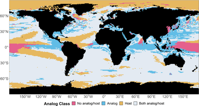
that more than one fourth (27%) of surface ocean pixels had no thermal analog, indicating that their unique climatic conditions would be lost by 2100 (Fig. 1). Most of these pixels were

found in northern oceans, which are affected by high warming rates21,22. The northern oceans mostly hosted thermal analogous conditions to those currently observed in more southern areas.

This finding was consistent with existing studies, indicating that species will have to move northward to meet their preferred climatic conditions11,12. Almost one fifth (19%) of pixels were

projected to experience novel climates in the future; consequently, these pixels could not host climatic conditions of the recent past. These pixels primarily occurred in the tropics,

likely reflecting the extreme climatic events of this zone23. About 4% of ocean pixels had no thermal analog, nor would they be thermal analog for other climates in the future. Most of these

pixels were located in the tropics (equatorial Pacific Ocean). OCEANIC AREAS THAT PROMOTE CLIMATE CONNECTIVITY As the global climate becomes warmer, future analogs of current local climatic

conditions may be found in distant areas14,16. For organisms to avoid passing through areas of highly dissimilar climatic conditions, trajectories between thermal analogs mostly pass

through specific sites that minimize climatic exposure. Across the seascape, pixels that could facilitate movement between thermal analogs were found to be spatially aggregated, covering

extensive marine areas; however, their extent and distribution varied among oceans and latitudes (Fig. 2a). These areas, which could contribute to climate connectivity under projected shifts

of ocean climate, were identified using current flow at each ocean pixel18. This metric quantifies the probability that a trajectory between thermal analogs passes through a given pixel.

Current flow was projected to be higher in northern areas (\({r}_{s}=0.70,p \, < \, 0.01\), Fig. 3a). Overall, oceans in the Northern Hemisphere (i.e., Arctic, north Pacific and north

Atlantic oceans) had higher current values, indicating that movement between analogs would become more intense in these oceans compared to oceans in the Southern Hemisphere

(\(H=19621,{df}=6,p \, < \, 0.01\); Supplementary Fig. S1). This phenomenon might be related to the higher warming rate of north21,22. Furthermore, extensive land mass in the north

constrained the trajectories between thermal analogs, eliminating potential routes. For instance, the highest metric values were found in areas located between North America and Asia (such

as the Bering Sea), at Gibraltar (which connects the Atlantic Ocean and the Mediterranean Sea), and at the Baltic Sea in Scandinavia. These areas are formed of narrow passages, where limited

alternative routes exist. Multiple sites near the equator had high path density, with this metric quantifying the number of optimal routes that pass over a pixel17 (Fig. 2b). Path density

had no latitudinal pattern (_r__s_ = −0.08, _p_ < 0.01) and was weakly correlated with current flow (\({r}_{s}=0.17,p \, < \, 0.01\)). As path density is based on the optimal routes

between thermal analogs, it could be a more representative metric for assessing connectivity potential for highly migratory species, while current flow accounts for multiple pathways, and

could be more suitable for species with limited dispersal capacity18. Many notable differences between the two metrics were observed in the oceans (Supplementary Figs. S1–2). For example,

multiple sites in the Indian Ocean had high path densities but relatively low current flow values. Still, certain marine regions (e.g., North Atlantic Ocean) and areas with narrow passages

(e.g., Bering Sea, Gibraltar) were identified as important by both metrics. In addition, multiple sites in the equatorial Pacific Ocean facilitated little to no movement between thermal

analogs for both metrics, mirroring evidence on high warming rates in this basin24 that will likely impede species dispersal. CLIMATIC VELOCITY At the tropical and subtropical regions of the

Western Atlantic Ocean, many pixels had high velocity but relatively low climatic exposure (Fig. 2c, d). Thus, while these sites had thermal analogs in distant areas, their trajectories

would pass over sites with conditions close to optimal thermal ranges. The topographical barriers in this region were limited to the land masses of South and Central America, providing

multiple pathways towards thermal analogs. Yet, for many tropical regions across the planet, the rate and magnitude of warming could generate novel climates25,26, potentially eliminating the

connectivity process. There is increasing evidence of widespread declines in marine tropical biodiversity27,28,29. Similarly, future climate, projections have revealed high rates of loss of

tropical species30,31. The physical barriers created by the land masses in the northern oceans of the planet, along with the higher warming rate in these areas21,22,32,33, resulted in a

latitudinal pattern in climatic velocity (_r__s_ = 0.59, _p_ < 0.01) and climatic exposure (_r__s_ = 0.63, _p_ < 0.01) (Fig. 2c, d). The few pixels in the Arctic Ocean that had thermal

analogs required longer (\(H=6105.3,{df}=6,p \, < \, 0.01\), Supplementary Fig. S3) and more exposed transitions (\(H=7858.5,{df}=6,p \, < \, 0.01\), Supplementary Fig. S4) compared

to the other oceans. Major changes to community composition in the Northern Hemisphere are projected in the future34,35,36, because the region will be exposed to high warming rate37. While

there are northern sites with thermal analogs, some species are likely to be further challenged by lower climatic connectivity. For instance, while species in North and Norwegian Seas track

analogous climatic conditions quickly, this might not be the case for species in the Barents Sea12, which is projected to be exposed to high warming37. In contrast, pixels in the Southern

Hemisphere have lower velocity and climatic exposure values, indicative of less distant thermal analogs, passing through similar climates during the transition. Approximately 14% of pixels

with thermal analogs had a climatic exposure value of zero, with most occurring in the Southern Hemisphere (Fig. 2d). Still, the tolerance of different marine organisms to warming and

changes to productivity, along with sea ice characteristics and seasonal dynamics, would further challenge their ability to track their suitable climatic conditions38. In particular, species

of great ecological significance in the Southern Hemisphere, such as Antarctic krill, are highly vulnerable to climate change, which will drive changes to their distributions39.

CONNECTIVITY BETWEEN MAJOR FISHING AREAS (MFAS) Large spatial variations were prevalent in connectivity patterns among MFAs, as defined based on the proportion of the surface expected to

have or become (i.e. host) a thermal analog by 2100. MFAs close to equator were projected to relatively have more analogs, while southern hemisphere MFAs had in general higher proportions of

areas with future thermal analogs than northern ones (Fig. 4). Moreover, two southern hemisphere MFAs, the Southeast Pacific Ocean and the Eastern Indian Ocean (i.e., No 87 and 57 in Fig. 

4b) hosted more thermal analogs (31.5 and 26% of total surface respectively) than other MFAs. Nonetheless, for all MFAs, future thermal analogs were mostly observed in long-distance areas.

For example, current local climate conditions of sites in the Northeast Pacific Ocean had their future analogs in the Northeast Atlantic Ocean (Supplementary Fig. S12). These findings on sea

surface climate connectivity patterns underline the fact that, for many species, possible range shifts would not be efficient enough to track and reach thermal analogous areas. BIODIVERSITY

HOTSPOTS AND THEIR FUTURE THERMAL ANALOGOUS SITES The analyses on key marine biodiversity areas further supported these concerns, as future thermal analogs were mostly found in thousands of

kilometers apart from the current biodiversity hotspots (Fig. 5). These long distances exceed dispersal capacities of most marine species40. Furthermore, the fact that the current hotspots

are mostly found close to coastal areas, while their future analogs are almost always located in the open sea, indicate that future thermal analogs may not serve as future habitat analogs

for the species, highlighting the potential risk for the perseveration of marine biodiversity within the following decades. FUTURE ENHANCEMENTS OF CLIMATE CONNECTIVITY METHODOLOGICAL

FRAMEWORK Methodological approaches permitting the efficient modeling of climate connectivity, while also considering narrow time-lag intervals when investigating future thermal analogs, are

lacking17. The methodology presented here could serve as a step towards addressing this challenge, providing the means to account for climate-driven species displacements and potential

movement pathways, in addition to short-term thermal barriers, which might limit the ability of organisms to migrate to maintain their thermal niche. Here, we used data from current and

future projections of ocean surface temperatures, based on the CMIP6 models. To our knowledge, these are the most accurate climate projections currently available at the global scale, with

slight improvements over the CMIP5 models41,42,43,44. Nevertheless, these models are subjected to biases; for example predictions on El-Nino warming pattern in the equatorial Pacific ocean,

indicate faster warming in the east than in the west45,46. These biases could potentially lead to an underestimation on connectivity status, as multiple pixels in this region were projected

to fail hosting climatic conditions of the recent past (Fig. 1). Similar biases are present for modeled historical data, such for the case of equatorial pacific cold tongue47, which could

also have an effect on the proper identification of future thermal analog pixels. However, the alternative use of historical observed data would not be suitable in our case, as their

production is based on a number of assumptions, leading to biases that differ from the ones in CMIP models. On the contrary, by using the same global circulation models (i.e. CMIP6) for both

present and future data, it is guaranteed that these biases are propagated equally across the entire time period studied48. Considering that each specific CMIP model has distinct

assumptions, sea surface connectivity patterns could be affected by the climatic model selected as sea surface input. To overcome this limitation, we selected an ensemble model that provides

mean temperature values from multiple models instead of a single one, mitigating the potential over- or under-estimation of sea surface temperature from specific models. Yet, although the

results of our analysis are valid in terms of surface thermal habitat, other factors such as ocean structure, currents, oxygen concentration, salinity and prey availability are also

important49,50. Additional environmental information could facilitate a more comprehensive approach that accounts for species specific preferences. More importantly, while sea surface

temperature is traditionally used to project climate-related patterns at different spatial and temporal scales51,52, and to explore a range of potential responses of marine organisms3,12,

the marine realm is inherently three-dimensional. Assuring vertical coherence of marine ecosystems against climate change impacts could prevent risking the disruption of trophic interactions

and reduce exposure to novel climates48,53. Within this framework, information on species observations, potential responses, and climate redistribution patterns across the three dimensions

should be considered54,55 to move towards future climate-smart conservation planning approaches and networks56. The methodological framework introduced in this paper could be applied at

various spatial scales and different depths, encouraging future studies to investigate multi-variable and multi-dimensional connectivity patterns. CONCLUSIONS To support conservation

planning, several tools have been developed to project potential climate-driven shifts of species distribution. For instance, ecological niche models57, metrics of the velocity of isotherm

shifts15,58, and spatial patterns of future thermal analogs16,59, offer projections of future redistribution of biodiversity. Many such spatial trajectories are now available and are being

used to assess conservation efficiency and policy recommendations54,60. Yet, our results demonstrate that delineating potential isotherm shifts based on distinct time slots of climate alone

(i.e., current and projected climatic niche, climate change velocity over distinct periods, thermal analogs) largely overlook the inherent dynamics of seascape climate. For example, while

the increased warming rate of the northern seas might force local species to exhibit certain movements to capture favorable climatic conditions, our findings on distant analogs, connected by

paths that are exposed to extreme climate, lead us to question the ability of the species to perform such movements successfully. The framework presented here provides a foundation on which

to explore the potential of the projected climate driven distribution shifts of marine organisms, under the dimension of climate connectivity. We, thus, call for future research that

incorporates the methods and outputs presented here towards providing a more comprehensive view of future range shifts in the marine environment. METHODS CLIMATE DATA To assess the climate

of the global ocean, we combined daily data of historical and future temperature projections from 11 ocean surface temperature models (Table S1) from Coupled Model Intercomparison Project

phase 6 (CMIP6)61. Initially, for each model, we used the daily data to calculate the minimum and maximum monthly data per year. To obtain a more comprehensive estimate of climatic

conditions for time intervals larger than a single year, we regrouped the yearly datasets into 30 five-year periods (hereafter, called periods). Then, we calculated the mean minimum and

maximum monthly data for each five-year period. To obtain an ensemble sea surface temperature model, we combined all 11 models by extracting the mean minimum and maximum monthly data per

period. This process resulted in 24 climatic layers per period (i.e., 12 for minimum and maximum monthly data, respectively). The data provided by the 11 ocean surface temperature models

were available on native grids, so they were transformed to a regular grid using the “akima” package in R. Then, the data were interpolated to a common grid of 1° × 1° resolution, using the

“resample” function in R, under bilinear interpolation, which is used for continuous variables. The time period studied here covered 150 years, extending from 1951 to 2100. Future

projections are based on the Shared Socioeconomic Pathways (SSP) 5–8.5 and 2–4.562. Climatic connectivity outputs, generated under the two SPPs, were then compared (see Supplementary Methods

 S1, Tables S3–S7, Figs. S6–S11 for details on this sensitivity analysis). To explore the sensitivity of our outputs to the climate scenarios used, we compared the connectivity patterns

between thermal analogous sites over short-term (2050), rather than long-term future climatic conditions (2100), under both SSP 2–4.5 and 5–8.5 scenarios. We also examined whether the length

of the periods affected our results, by repeating the analysis with 10-year periods instead of 5-year periods. BIOCLIMATIC VARIABLES For each period, we calculated nine bioclimatic

variables that express seasonal trends and extreme temperature values (Table S2). These variables were calculated based on the minimum and maximum monthly temperature data obtained by our

ensemble temperature model (see Climate data section). To reduce the number of variables, while maintaining the information provided, we performed a principal component analysis. Our

variables fulfilled the requirements for this analysis, as they consisted of a large number of records (i.e., 42864 pixels), were significantly correlated under the Pearson correlation

coefficient (\(p \, < \, 0.05\)), with mostly high correlation values, indicating linearity, and there were few outliers. We reduced the bioclimatic variables to two principal components

(hereafter, \({PC}1\) and \({PC}2\), Supplementary Fig. S5), which explained 93.3% of the variance in the original variables. Following this process, we generated 60 climate layers (i.e.,

two principal components for each period). DEFINING CLIMATES The values of the two principal components were scaled based on the minimum and maximum values of the first period (i.e.,

1951–1955), using the following formula17: $$P{C}_{i}^{{\prime} }=1+99 * \frac{P{C}_{i}-min\{P{C}_{1}\}}{max\{P{C}_{1}\}-min\{P{C}_{1}\}}$$ (1) where \({{PC}}_{i}\) denotes a principal

component for period \(i\). Using this formula, the principal component values in the first period were scaled in the range of [1, 100], while those for other periods could fall out of this

range, indicative of novel climates. To classify the principal component values, we created two sets of bins, one per component. The bin centers were integer values, of \(\pm 0.5\) width,

covering all \({PC}\) scaled values. There were 116 bins for \({PC}1\) and 104 bins for \({PC}2\), resulting in 12064 possible combinations. These bin combinations were used to define

climate. We identified 2780 different climates in the first period. THERMAL ANALOGS AND THEIR CONNECTIONS A pixel was considered to have a thermal analog if its thermal conditions in the

first period (i.e., 1951–1955) was observed in the last period (i.e., period 30; 2096–2100), either on the same pixel or a different pixel. Following this process, each pixel was classified

into one of four classes: (i) will have a thermal analog and will host past thermal conditions in the future; (ii) will have a thermal analog but will not host past thermal conditions in the

future; (iii) will not have a thermal analog but will host past thermal conditions in the future; and (iv) will not have a thermal analog and will not host past thermal conditions in the

future. To quantify the exposure of trajectories between thermal analogs to dissimilar climates, we constructed cost surfaces. Following Carroll et al.17, cost surfaces indicate the climatic

dissimilarity of the seascape for a given climate (i.e., difference in \({PC}1\) and \({PC}2\) values). For each unique climate, we constructed 30 cost surfaces (one per period). The total

cost for pixel \(k\) is: $${cost}\left(k\right)=1+p* \left|{PC}1-{PC}1\left(k\right)\right|+p* {{{{{\rm{|}}}}}}{PC}2-{PC}2(k){{{{{\rm{|}}}}}}$$ (2) where \({PC}1\) and \({PC}2\) denote the

\({PC}\) values of the specific climate; \({PC}1(k)\) and \({PC}2(k)\) denote the \({PC}\) values of pixel \(k\); and \(p\) is the dissimilarity penalty. In our case, \(p=2\)16,17,

indicating that a unit of difference between the scaled \({PC}\) values increases the cost by 2. The sensitivity of our results to cost penalty was also examined, by using alternative cost

values, which did not alter the observed patterns in connectivity (see Supplementary Table S6). The final climate cost surface, which integrated all periods, was derived as the minimum cost

per pixel from all periods. CONNECTIVITY METRICS To quantify climate connectivity between thermal analogous ocean surface pixels, we used four metrics. These metrics used the cost surfaces

to quantify the extent to which the seascape impedes connectivity between pixels. The first two metrics were current flow18 and path density17 and were used to evaluate pixels based on the

extent to which they facilitates movement between thermal analogs. Current flow is a metric derived from circuit theory18. It models the displacement of an individual that moves randomly on

a raster mosaic between two thermal analogs. The movement from one pixel towards its considered future analog is based on a cost surface, with low-cost pixels having a higher probability to

be selected as the next movement step. The final output is a current flow map, indicating the pixel-wise probability that the trajectory between the thermal analogs passes through it18. We

used this metric as an ensemble for all trajectories, quantifying the overall pixel-wise probability that a trajectory between any pair of thermal analogs passes through a given pixel. Path

density17 is based on least-cost path algorithm19. Based on the cost surface, this algorithm extracts the trajectory between two thermal analogs with the minimum cumulative cost. This

trajectory has two attributes, its length and its cumulative cost19. Path density measures the number of these trajectories that cross a pixel. Therefore, for a given pixel, the key

difference between the two metrics is that for current flow estimation, we assume that an individual organism moves randomly, based on climatic dissimilarity, whereas for path density

calculations, we only consider the trajectories that minimize climatic exposure (i.e., least-cost paths)19. Path density accounts for specific trajectories along which organisms move with

prior knowledge of the climate, and thus traverse through the seascape, while minimizing climatic exposure. Current flow, given the limited knowledge of the seascape, is used to quantify

movement towards all thermal analog pixels. Conversely, path density only accounts for the trajectories of a pixel to its thermal analog with the minimum cumulative cost (i.e., the minimum

climatic exposure). The other two metrics used here were minimum exposure distance (MED)16 and minimum cumulative exposure (MCE)16. These metrics indicate the effort required for an

individual (i.e., species) to reach the thermal analog. These two metrics were only available for pixels with thermal analogs. To calculate these metrics for a given pixel, we first

extracted the trajectory to its thermal analog that minimizes climatic exposure, by using the least-cost path algorithm19. MED quantified climatic velocity, which is defined as the length

attribute of the extracted trajectory. MCE is a complementary metric that is used to quantify the exposure to dissimilar climates during this transition, being equal to the difference

between the trajectory’s cumulative cost and its length16. When a pixel has multiple thermal analogs, the values maintained are those obtained from the trajectory with the lowest climatic

exposure. We also used these metrics to examine the connectivity status at the ocean level. We extracted ocean boundaries from the International Hydrographic Organization (IHO) Sea Areas v3

(www.marineregions.com). For all seven ocean basins (i.e., Arctic, north Pacific, south Pacific, north Atlantic, south Atlantic, Indian, and Southern), we identified the surface pixels

within their boundary. Then, we conducted four Kruskall–Wallis H tests (one per metric) to examine potential differences in the distribution of metric values among the oceans. CONNECTIVITY

BETWEEN MARINE AREAS To identify the location of the future analogs of broader marine areas, we partitioned the ocean realm based on the Major Fishing Areas (MFAs) of the Food and

Agriculture Organization (FAO) categorization. We used graph theory63,64 to describe the properties of the climate connectivity among the MFA network. A graph consists of a set of nodes

(here the MFAs), with links between them depicting the strength of their connection63,64. This graph is directed, which means that considering two areas, namely A and B, the link from A to B

is not necessarily equal to the link from B to A, depending on which area is considered as the present climate and which one is considered as its future analog. Since future analogs of

local climate conditions could also be identified within the same MFA, links from an area towards itself were also included. To evaluate the links between each pair of MFAs, we quantified

(i) the percentage of pixels in the first MFA that have a future analog in the second MFA and (ii) the percentage of pixels in the second MFA that will host analogs of the first MFA.

Finally, we accounted for the mean percentage of pixels with analogs, as well as the mean percentage of pixels that will host analogs per MFA. THERMAL ANALOGS OF BIODIVERSITY HOTSPOTS We

considered six distinct marine biodiversity hotspots, as delineated by Ramirez et al.20, based on the distributions of 2183 marine species (fish, marine mammals, and seabirds). We

interpolated the biodiversity hotspots data from the initial grid of 0.5° × 0.5° resolution to a grid of 1° × 1° resolution, using the “resample” function in R, under nearest neighbor

interpolation. We identified the thermal analogs of the pixels of each of the six hotspots, while in case of multiple analogs per pixel, we maintained the one having the trajectory that

minimizes the exposure to dissimilar climates. DATA AVAILABILITY Data on sea surface temperature models from CMIP6 was extracted from Earth System Grid Federation (ESGF) node in Deutsches

Klimarechenzentrum (DKRZ). Ocean boundaries were extracted from the International Hydrographic Organization (IHO) Sea Areas v3 (www.marineregions.com). Major Fishing Areas (MFAs) were

extracted from the Food and Agriculture Organization (FAO) (www.marineregions.com). Data on biodiversity hotspots were extracted from the Spanish National Research Council [Consejo Superior

de Investigaciones Científicas (CSIC)] digital repository. Source data for figures presented in this manuscript are available in Figshare: Figures 1–3:

https://doi.org/10.6084/m9.figshare.20747605.v2 Figure 4: https://doi.org/10.6084/m9.figshare.20747653.v2 Figure 5: https://doi.org/10.6084/m9.figshare.20748151.v2. CODE AVAILABILITY Code

used to calculate the metrics is available in Figshare: https://doi.org/10.6084/m9.figshare.20748301.v3. REFERENCES * Sydeman, W. J., Poloczanska, E., Reed, T. E. & Thompson, S. A.

Climate change and marine vertebrates. _Science (1979)_ 350, 772–777 (2015). CAS  Google Scholar  * Lind, S., Ingvaldsen, R. B. & Furevik, T. Arctic warming hotspot in the northern

Barents Sea linked to declining sea-ice import. _Nat. Clim. Chang._ 8, 634–639 (2018). Article  Google Scholar  * Pinsky, M. L., Selden, R. L. & Kitchel, Z. J. Climate-driven shifts in

marine species ranges: scaling from organisms to communities. _Ann. Rev. Mar. Sci._ 12, 153–179 (2020). Article  Google Scholar  * Cheng, L., Abraham, J., Hausfather, Z. & Trenberth, K.

E. How fast are the oceans warming? _Science (1979)_ 363, 128–129 (2019). CAS  Google Scholar  * Henson, S. A. et al. Rapid emergence of climate change in environmental drivers of marine

ecosystems. _Nat Commun._ 8, 1–9 (2017). Article  Google Scholar  * Babcock, R. C. et al. Severe continental-scale impacts of climate change are happening now: extreme climate events impact

marine habitat forming communities along 45% of Australia’s coast. _Front Mar Sci._ 6, 411 (2019). Article  Google Scholar  * Smale, D. A. et al. Marine heatwaves threaten global

biodiversity and the provision of ecosystem services. _Nat Clim Chang._ 9, 306–312 (2019). Article  Google Scholar  * Perry, A. L., Low, P. J., Ellis, J. R. & Reynolds, J. D. Climate

change and distribution shifts in marine fishes. _Science (1979)_ 308, 1912–1915 (2005). CAS  Google Scholar  * Last, P. R. et al. Long‐term shifts in abundance and distribution of a

temperate fish fauna: a response to climate change and fishing practices. _Glob. Ecol. Biogeogr._ 20, 58–72 (2011). Article  Google Scholar  * Sorte, C. J. B., Williams, S. L. & Carlton,

J. T. Marine range shifts and species introductions: comparative spread rates and community impacts. _Glob. Ecol. Biogeogr._ 19, 303–316 (2010). Article  Google Scholar  * Fossheim, M. et

al. Recent warming leads to a rapid borealization of fish communities in the Arctic. _Nat. Clim. Chang._ 5, 673–677 (2015). Article  Google Scholar  * Lenoir, J. et al. Species better track

climate warming in the oceans than on land. _Nat. Ecol. Evol._ 4, 1044–1059 (2020). Article  Google Scholar  * Nuñez, T. A. et al. Connectivity planning to address climate change. _Conserv.

Biol._ 27, 407–416 (2013). Article  Google Scholar  * Burrows, M. T. et al. Geographical limits to species-range shifts are suggested by climate velocity. _Nature_ 507, 492–495 (2014).

Article  CAS  Google Scholar  * Hamann, A., Roberts, D. R., Barber, Q. E., Carroll, C. & Nielsen, S. E. Velocity of climate change algorithms for guiding conservation and management.

_Glob. Chang. Biol._ 21, 997–1004 (2015). Article  Google Scholar  * Dobrowski, S. Z. & Parks, S. A. Climate change velocity underestimates climate change exposure in mountainous

regions. _Nat. Commun._ 7, 1–8 (2016). Article  Google Scholar  * Carroll, C., Parks, S. A., Dobrowski, S. Z. & Roberts, D. R. Climatic, topographic, and anthropogenic factors determine

connectivity between current and future climate analogs in North America. _Glob. Chang. Biol._ 24, 5318–5331 (2018). Article  Google Scholar  * McRae, B. H., Dickson, B. G., Keitt, T. H.

& Shah, V. B. Using circuit theory to model connectivity in ecology, evolution, and conservation. _Ecology_ 89, 2712–2724 (2008). Article  Google Scholar  * Adriaensen, F. et al. The

application of ‘least-cost’modelling as a functional landscape model. _Landsc Urban Plan_ 64, 233–247 (2003). Article  Google Scholar  * Ramírez, F., Afán, I., Davis, L. S. & Chiaradia,

A. Climate impacts on global hot spots of marine biodiversity. _Sci. Adv._ 3, e1601198 (2017). Article  Google Scholar  * Ruela, R., Sousa, M. C., deCastro, M. & Dias, J. M. Global and

regional evolution of sea surface temperature under climate change. _Glob. Planet Change_ 190, 103190 (2020). Article  Google Scholar  * Tamarin-Brodsky, T., Hodges, K., Hoskins, B. J. &

Shepherd, T. G. Changes in Northern Hemisphere temperature variability shaped by regional warming patterns. _Nat. Geosci._ 13, 414–421 (2020). Article  CAS  Google Scholar  * Barlow, J. et

al. The future of hyperdiverse tropical ecosystems. _Nature_ 559, 517–526 (2018). Article  CAS  Google Scholar  * Collins, M. et al. The impact of global warming on the tropical Pacific

Ocean and El Niño. _Nat. Geosci._ 3, 391–397 (2010). Article  CAS  Google Scholar  * Collin, R., Rebolledo, A. P., Smith, E. & Chan, K. Y. K. Thermal tolerance of early development

predicts the realized thermal niche in marine ectotherms. _Funct. Ecol._ 35, 1679–1692 (2021). Article  CAS  Google Scholar  * Nguyen, K. D. T. et al. Upper temperature limits of tropical

marine ectotherms: global warming implications. _PLoS ONE_ 6, e29340 (2011). Article  CAS  Google Scholar  * Wernberg, T. et al. An extreme climatic event alters marine ecosystem structure

in a global biodiversity hotspot. _Nat. Clim. Chang._ 3, 78–82 (2013). Article  Google Scholar  * Chaudhary, C., Saeedi, H. & Costello, M. J. Bimodality of latitudinal gradients in

marine species richness. _Trends Ecol. Evol._ 31, 670–676 (2016). Article  Google Scholar  * Oremus, K. L. et al. Governance challenges for tropical nations losing fish species due to

climate change. _Nat Sustain_ 3, 277–280 (2020). Article  Google Scholar  * Jones, M. C. & Cheung, W. W. L. Multi-model ensemble projections of climate change effects on global marine

biodiversity. _ICES J. Mar. Sci._ 72, 741–752 (2015). Article  Google Scholar  * Blowes, S. A. et al. The geography of biodiversity change in marine and terrestrial assemblages. _Science

(1979)_ 366, 339–345 (2019). CAS  Google Scholar  * Li, J. & Thompson, D. W. J. Widespread changes in surface temperature persistence under climate change. _Nature_ 599, 425–430 (2021).

Article  CAS  Google Scholar  * Kornhuber, K. & Tamarin‐Brodsky, T. Future changes in Northern Hemisphere summer weather persistence linked to projected Arctic warming. _Geophys. Res.

Lett._ 48, e2020GL091603 (2021). Article  Google Scholar  * Molinos, J. G. et al. Climate velocity and the future global redistribution of marine biodiversity. _Nat. Clim. Chang._ 6, 83–88

(2016). Article  Google Scholar  * Burrows, M. T. et al. Ocean community warming responses explained by thermal affinities and temperature gradients. _Nat. Clim. Chang._ 9, 959–963 (2019).

Article  Google Scholar  * Pimiento, C. et al. Functional diversity of marine megafauna in the Anthropocene. _Sci. Adv._ 6, eaay7650 (2020). Article  CAS  Google Scholar  * Albouy, C. et al.

Global vulnerability of marine mammals to global warming. _Sci. Rep._ 10, 1–12 (2020). Google Scholar  * Constable, A. J. et al. Climate change and Southern Ocean ecosystems I: how changes

in physical habitats directly affect marine biota. _Glob. Chang. Biol._ 20, 3004–3025 (2014). Article  Google Scholar  * Rogers, A. D. et al. Antarctic futures: an assessment of

climate-driven changes in ecosystem structure, function, and service provisioning in the Southern Ocean. _Ann. Rev. Mar. Sci._ 12, 87–120 (2020). Article  CAS  Google Scholar  * Lester, S.

E., Ruttenberg, B. I., Gaines, S. D. & Kinlan, B. P. The relationship between dispersal ability and geographic range size. _Ecol. Lett._ 10, 745–758 (2007). Article  Google Scholar  *

Grose, M. R. et al. Insights from CMIP6 for Australia’s future climate. _Earths Future_ 8, e2019EF001469 (2020). Article  Google Scholar  * McKenna, S., Santoso, A., Gupta, A., sen,

Taschetto, A. S. & Cai, W. Indian Ocean Dipole in CMIP5 and CMIP6: characteristics, biases, and links to ENSO. _Sci. Rep._ 10, 1–13 (2020). Article  Google Scholar  * You, Q. et al.

Temperature dataset of CMIP6 models over China: evaluation, trend and uncertainty. _Clim. Dyn._ 57, 17–35 (2021). Article  Google Scholar  * Richter, I. & Tokinaga, H. An overview of the

performance of CMIP6 models in the tropical Atlantic: mean state, variability, and remote impacts. _Clim. Dyn._ 55, 2579–2601 (2020). Article  Google Scholar  * Cai, W. et al. Changing El

Niño–Southern Oscillation in a warming climate. _Nat. Rev. Earth Environ._ 2, 628–644 (2021). Article  Google Scholar  * Power, S. et al. Decadal climate variability in the tropical Pacific:

characteristics, causes, predictability, and prospects. _Science (1979)_ 374, eaay9165 (2021). CAS  Google Scholar  * Li, G. & Xie, S.-P. Tropical biases in CMIP5 multimodel ensemble:

the excessive equatorial Pacific cold tongue and double ITCZ problems. _J. Clim._ 27, 1765–1780 (2014). Article  Google Scholar  * Brito-Morales, I. et al. Climate velocity reveals

increasing exposure of deep-ocean biodiversity to future warming. _Nat. Clim. Chang._ 10, 576–581 (2020). Article  CAS  Google Scholar  * Robinson, L. M. et al. Pushing the limits in marine

species distribution modelling: lessons from the land present challenges and opportunities. _Glob. Ecol. Biogeogr._ 20, 789–802 (2011). Article  Google Scholar  * Chen, Y. et al. Estimating

seasonal habitat suitability for migratory species in the Bohai Sea and Yellow Sea: a case study of Tanaka’s snailfish (Liparis tanakae). _Acta Oceanologica Sinica_ 1–9 (2022). * Almpanidou,

V., Markantonatou, V. & Mazaris, A. D. Thermal heterogeneity along the migration corridors of sea turtles: implications for climate change ecology. _J Exp Mar Biol Ecol_ 520, 151223

(2019). Article  Google Scholar  * Plecha, S. M. & Soares, P. M. M. Global marine heatwave events using the new CMIP6 multi-model ensemble: from shortcomings in present climate to future

projections. _Environ. Res. Lett._ 15, 124058 (2020). Article  Google Scholar  * Brito-Morales, I. et al. Towards climate-smart, three-dimensional protected areas for biodiversity

conservation in the high seas. _Nat. Clim. Chang._ 1–6 (2022). * Arafeh‐Dalmau, N. et al. Incorporating climate velocity into the design of climate‐smart networks of marine protected areas.

_Methods Ecol. Evol._ 12, 1969–1983 (2021). Article  Google Scholar  * McBride, M. M. et al. Antarctic krill Euphausia superba: spatial distribution, abundance, and management of fisheries

in a changing climate. _Mar. Ecol. Prog. Ser._ 668, 185–214 (2021). Article  Google Scholar  * Doxa, A., Kamarianakis, Y. & Mazaris, A. D. Spatial heterogeneity and temporal stability

characterize future climatic refugia in Mediterranean Europe. _Glob. Chang Biol._ (2022). * Melo-Merino, S. M., Reyes-Bonilla, H. & Lira-Noriega, A. Ecological niche models and species

distribution models in marine environments: a literature review and spatial analysis of evidence. _Ecol. Modell._ 415, 108837 (2020). Article  Google Scholar  * Loarie, S. R. et al. The

velocity of climate change. _Nature_ 462, 1052–1055 (2009). Article  CAS  Google Scholar  * García Molinos, J. et al. Improving the interpretability of climate landscape metrics: an

ecological risk analysis of Japan’s Marine Protected Areas. _Glob. Chang. Biol._ 23, 4440–4452 (2017). Article  Google Scholar  * Sala, E. et al. Protecting the global ocean for

biodiversity, food and climate. _Nature_ 592, 397–402 (2021). Article  CAS  Google Scholar  * Eyring, V. et al. Overview of the Coupled Model Intercomparison Project Phase 6 (CMIP6)

experimental design and organization. _Geosci. Model Dev._ 9, 1937–1958 (2016). Article  Google Scholar  * Riahi, K. et al. The shared socioeconomic pathways and their energy, land use, and

greenhouse gas emissions implications: an overview. _Global Environ Change_ 42, 153–168 (2017). Article  Google Scholar  * Urban, D. & Keitt, T. Landscape connectivity: a graph‐theoretic

perspective. _Ecology_ 82, 1205–1218 (2001). Article  Google Scholar  * Petsas, P., Almpanidou, V. & Mazaris, A. D. Landscape connectivity analysis: new metrics that account for patch

quality, neighbors’ attributes and robust connections. _Landsc Ecol._ 36, 3153–3168 (2021). Article  Google Scholar  Download references ACKNOWLEDGEMENTS A.D., V.A., and A.D.M. were

supported from the FutureMARES project that has received funding from the European Union’s Horizon 2020 research and innovation programme under grant agreement No 869300. P.P. was supported

by the Hellenic Foundation for Research and Innovation (HFRI) under the HFRI PhD Fellowship grand (Fellowship Number: 1018). AUTHOR INFORMATION AUTHORS AND AFFILIATIONS * Department of

Ecology, School of Biology, Aristotle University of Thessaloniki, Thessaloniki, Greece Panagiotis Petsas, Aggeliki Doxa, Vasiliki Almpanidou & Antonios D. Mazaris * Institute of Applied

and Computational Mathematics, Foundation for Research and Technology-Hellas (FORTH), Heraklion, Crete, Greece Aggeliki Doxa Authors * Panagiotis Petsas View author publications You can also

search for this author inPubMed Google Scholar * Aggeliki Doxa View author publications You can also search for this author inPubMed Google Scholar * Vasiliki Almpanidou View author

publications You can also search for this author inPubMed Google Scholar * Antonios D. Mazaris View author publications You can also search for this author inPubMed Google Scholar

CONTRIBUTIONS A.D.M. and P.P. conceived the ideas and designed the methodology. P.P. led the analysis and coding. V.A. and A.D. contributed to ecological knowledge and statistical analyses.

All authors contributed critically to the drafts and gave final approval for publication. CORRESPONDING AUTHOR Correspondence to Panagiotis Petsas. ETHICS DECLARATIONS COMPETING INTERESTS

The authors declare no competing interests. PEER REVIEW PEER REVIEW INFORMATION _Communications Earth & Environment_ thanks Isaac Brito-Morales and the other, anonymous, reviewer(s) for

their contribution to the peer review of this work. Primary Handling Editors: Clare Davis and Alienor Lavergne. Peer reviewer reports are available. ADDITIONAL INFORMATION PUBLISHER’S NOTE

Springer Nature remains neutral with regard to jurisdictional claims in published maps and institutional affiliations. SUPPLEMENTARY INFORMATION SUPPLEMENTARY MATERIAL PEER REVIEW FILE

RIGHTS AND PERMISSIONS OPEN ACCESS This article is licensed under a Creative Commons Attribution 4.0 International License, which permits use, sharing, adaptation, distribution and

reproduction in any medium or format, as long as you give appropriate credit to the original author(s) and the source, provide a link to the Creative Commons license, and indicate if changes

were made. The images or other third party material in this article are included in the article’s Creative Commons license, unless indicated otherwise in a credit line to the material. If

material is not included in the article’s Creative Commons license and your intended use is not permitted by statutory regulation or exceeds the permitted use, you will need to obtain

permission directly from the copyright holder. To view a copy of this license, visit http://creativecommons.org/licenses/by/4.0/. Reprints and permissions ABOUT THIS ARTICLE CITE THIS

ARTICLE Petsas, P., Doxa, A., Almpanidou, V. _et al._ Global patterns of sea surface climate connectivity for marine species. _Commun Earth Environ_ 3, 240 (2022).

https://doi.org/10.1038/s43247-022-00569-5 Download citation * Received: 28 May 2022 * Accepted: 26 September 2022 * Published: 14 October 2022 * DOI:

https://doi.org/10.1038/s43247-022-00569-5 SHARE THIS ARTICLE Anyone you share the following link with will be able to read this content: Get shareable link Sorry, a shareable link is not

currently available for this article. Copy to clipboard Provided by the Springer Nature SharedIt content-sharing initiative