The influence of administrative border on the spatial correlation of house prices: evidence from china

ABSTRACT This paper empirically examines the spatial correlation differences and mechanisms of housing prices in prefecture-level cities, considering the influence of administrative

boundaries. Using an extended spatial Durbin model and panel data from 292 prefecture-level cities in China between 2000 and 2013, the study identifies the attributes and stage

characteristics of real estate. The results indicate a significant spatial correlation in housing prices between neighboring prefecture-level cities, with inter-provincial administrative

boundaries reducing the spatial correlation between these cities by 62.11%. Further research reveals significant changes in the spatial correlation of housing prices following the 2007

subprime mortgage crisis, with the transformation of real estate’s dominant attributes being the primary reason for these changes. SIMILAR CONTENT BEING VIEWED BY OTHERS INTRA-URBAN HOUSE

PRICES IN MADRID FOLLOWING THE FINANCIAL CRISIS: AN EXPLORATION OF SPATIAL INEQUALITY Article Open access 24 April 2024 SPATIAL HETEROGENEITY ANALYSIS OF BIASED LAND RESOURCE SUPPLY POLICIES

ON HOUSING PRICES AND INNOVATION EFFICIENCY Article Open access 10 September 2024 THE TIME-VARYING IMPACT OF UNCERTAINTY SHOCKS ON THE CO-MOVEMENT OF REGIONAL HOUSING PRICES OF THE UNITED

KINGDOM Article Open access 12 February 2025 INTRODUCTION Housing is a basic need for human survival and an important source of residents’ happiness (Lin et al., 2012), as well as an

inevitable requirement for building a well-off society. At the same time, the excessively strong investment attributes of housing and the overly rapid rise in house prices often lead to a

series of socioeconomic problems such as housing price bubbles, weakened technological innovation, and the inhibition of long-term economic growth (Zhang et al., 2016; Wang and Rong, 2014;

Chen et al., 2018). In this regard, since the Central Economic Work Conference in December 2016, President Xi has repeatedly proposed the position that ‘houses are for living, not for

speculation’. However, because it is often difficult to separate the consumption and investment attributes of real estate (Yang et al., 2014b), existing studies have failed to explore the

changes in house prices from the perspective of their attributes, let alone identify the dominant attributes of housing at different stages of development. So, how to better distinguish the

consumption attributes and investment attributes of real estate, and identify the dominant attributes of real estate in different development stages? What is the internal root of the

regional housing price difference characterization? Is there a certain correlation between the attributes of real estate? The exploration of these problems is of great significance to the

identification of real estate attributes, the implementation of long-term real estate management mechanism, and the sustainable development of social economy. Theoretically, the dual

attributes of housing refer to the two functions of satisfying residents’ consumption and investment demands, and under different attributes, house prices show differentiated

characteristics. For example, the consumption attribute makes house prices have obvious regional differences, while the investment attribute is likely to cause house prices to deviate from

economic fundamentals (Liang and Gao, 2007). However, no matter which attribute real estate takes on, it will cause spatial correlation in house prices (He and Yang, 2016). Currently,

theoretical studies, represented by the ripple effect, have explored the causes of the spatial correlation of house prices from several aspects (Meen, 1996; Wang et al., 2008; Lv and Liu,

2019). Nevertheless, the spatial correlation differences and formation mechanisms of house prices under the dual attributes are still not examined. In fact, the ‘dual attributes’ of real

estate and administrative divisions are the root causes of the spatial heterogeneity of housing prices. Therefore, based on the spatial correlation differences of house prices within and

between provinces, the stage characteristics and attributes of real estate can be identified by using the population flow mechanism, capital flow mechanism, and information flow mechanism

that lead to the spatial correlation of house prices. In this regard, this paper discusses how the administrative boundary affects the formation mechanism and functional differences in the

spatial correlation of regional housing prices under the consumption and investment attributes. Furthermore, the extended spatial Durbin model (ESDM) is applied to identify the housing

attributes in each period. The full-sample study finds that housing has both consumption and investment attributes, and there is spatial correlation in house prices among neighboring

prefectural cities, and provincial administrative boundaries have a shielding effect on the spatial correlation of house prices. Moreover, the sub-sample study found that before 2008,

housing was dominated by the consumption attribute, and the spatial correlation of house prices in prefectural cities was significantly different within and between provinces. After 2008,

the investment attribute became dominant, and the spatial correlation of house prices in prefectural-level cities significantly existed both within and between provinces, and there were no

significant differences between the two. This paper has the following contributions: firstly, based on the influence of administrative boundaries, the spatial correlation and mechanisms of

house prices are examined for the first time from the perspective of dual attributes, and the intrinsic relationship between real estate attributes and the spatial correlation of regional

house prices is clarified. Secondly, by extending the existing spatial econometric models and estimation methods, an extended spatial Durbin model that can be used to identify the spatial

correlation of regional house prices and its consistent estimators has been developed. Thirdly, based on the panel data of Chinese prefecture-level cities from 2000 to 2013, the dominant

attributes of real estate at different stages are identified. The remainder of this paper is organized as follows: Section 2 reviews the relevant literature. Section 3 studies the

relationship between the real estate attributes and spatial correlation of house prices. Section 4 introduces the empirical strategy and data. Section 5 demonstrates the baseline results.

Section 6 conducts the robustness tests. Section 7 draws conclusions. LITERATURE REVIEW Since the 1980s, scholars have been exploring the attributes of housing, and it is generally believed

that housing has both consumption and investment attributes (Zhou, 2007; Zhang, 2017; Sebastien, 2010); that is, a house can be both a consumer good to meet people’s living needs and a

capital asset to fulfill individual investment demands. The dual attributes of housing make house prices move in a different manner from other commodities and financial assets (Henderson and

Ioannides, 1983; Kuang, 2010; Li et al., 2016). Past studies on house prices and their fluctuations have focused on two aspects: regional differences and spatial correlation. Housing prices

and their fluctuations show regional differences mainly because of the consumption attributes of housing (Liang and Gao, 2007). When studying regional differences in house prices and their

fluctuations, scholars often default to the consumption attribute of housing and explain them in terms of demand-side, supply-side, and non-market-side factors. Resident income, population

and structure are considered as demand-side factors (Muellbauer and Murphy,1997; Liang and Gao, 2007; Takáts, 2012; Xu and Wu, 2019), while land price and housing construction cost are

considered supply-side factors (Raymond, 1988; Shen and Liu, 2004; Kuang, 2005; Sirmans et al., (2005)). Regulations, administrative levels, and urban transportation accessibility are

considered non-market-side factors (Jarociński and Smets, 2008; Zhou and Wu, 2009; Jia and Ge, 2015; Huang et al. 2018; Fan et al. 2018). However, house prices are spatially correlated when

houses only play the role of consumption assets. In fact, under the dual attributes, the behavior of buyers, investors, or speculators in the property market can lead to spatial correlation

of house prices (He and Yang, 2016). Therefore, when discussing the spatial correlation of house prices and their fluctuations, scholars usually do not distinguish between the dual

attributes. At present, the Ripple Effect is the main theory used to analyze the spatial correlation of regional house prices. The ripple effect suggests that changes in house prices in some

areas will cause sequential changes in house prices in neighboring areas, just like ripples in water. Household migration, transaction costs, search costs, wealth transfer, spatial

arbitrage, lead-lag relationship of influencing factors and spatial heterogeneity are considered as the main reasons for the ripple effect (Meen, 1996; Wang et al., 2008). Based on the

ripple effect, the spatial correlation of regional house prices has also been widely investigated with three main types of empirical tests. First, the long-term convergence and interaction

causality of regional house prices are analyzed by using cointegration tests, causality tests, and impulse response functions. Gupta and Miller (2012) used Granger causality test to test the

regional interaction causality of real estate prices in the United States. Huang et al. (2009) verified the linkage effect of housing prices in major cities in China based on co-integration

and vector error correction model. Second, a linear regression model is used to examine the interaction of house prices between two regions by using house prices in one region as the

explanatory variable for house prices in the other region or the ratio of house prices in two regions as the explained variable. Hughes and McCormick (1994) directly used the ratio of house

prices in the south and north of the UK as the explained variable to study the correlation between house prices in the north and south of the UK. Holmes and Grimes (2008) used the housing

price data of the United Kingdom from 1973 to 2006 as a sample. After separating the main factors through principal component analysis, they found that housing prices in various regions of

the United Kingdom showed a single long-term equilibrium trend. Third, a spatial weighting matrix is introduced, and a spatial econometric model is established to capture the regional

interaction of house prices through spatial autocorrelation. Holly et al. (2011) and Brady (2011) used spatial econometric models to examine the spatial correlation of regional real estate

prices in the United States. Wang (2012), Ding and Ni (2015) verified the spatial autocorrelation of China’s regional housing prices based on the spatial panel model. In summary, housing

attribute classification and house price characteristics have received widespread attention. However, when studying housing attributes, existing studies have only theoretically elaborated on

them without empirical testing. When studying house prices, previous studies have either explored their specific characteristics (e.g., regional difference) by assuming a certain attribute

or directly analyzed their performance characteristics (e.g., spatial correlation) without considering the attribute. Based on the boundary effectsFootnote 1, this paper uses an extended

spatial Durbin model to identify the attribute representations of Chinese real estate at different stages from the perspective of the intra-provincial and inter-provincial correlation of

house prices. THEORETICAL MECHANISMS In recent years, with the boom of China’s real estate, the spatial correlation of house prices has been widely studied (Wang et al., 2008; Wang, 2012;

Ding and Ni, 2015). The main reasons for this include population mobility, capital mobility and information mobility (Lv, and Liu, 2019). However, whether these three factors are effective

is related to housing attributes, which has not been further explored by scholars due to the inseparability of the dual attributes (Yang et al., 2014b). This section explores the mechanism

and heterogeneity of the spatial association of house prices under different attributes (consumption attributes or investment attributes). CONSUMPTION ATTRIBUTE AND THE SPATIAL CORRELATION

OF HOUSE PRICES When housing serves the role of a consumption attribute, the buyers of housing are mainly real home-seekers with the purpose of living, including immigrant demand,

improvement demand, and renewal demand (Gao, 2015). Thus, housing prices are mainly determined by basic factors such as urban population, residents’ income, and construction costs (Green,

1999; Shen and Liu, 2004; Liang and Gao, 2006). At this stage, the population mobility mechanism is the main reason for the spatial correlation of house prices between cities. The population

mobility mechanism refers to the fact that when the house price of a city continues to rise, the population tends to migrate from high-price cities to low-price cities due to the cost of

living, which leads to the increase in house prices in low-price cities, forming a spatial linkage of house prices between cities. Housing expenditure accounts for a high proportion of the

cost of living (Zhang et al., 2012) and is an important factor influencing labor mobility (Zhang et al., 2017). High housing prices directly affect people’s quality of life and migration

decisions. The social phenomenon that began to emerge around 2010 is a good example of the exodus from the first-tier cities. Many young people chose to leave first-tier cities with high

housing prices because of housing pressure. As more people moved in, the demand for housing in low-cost cities increased, which led to a continuous rise in housing prices (Lu et al., 2014;

Li et al., 2017; He et al., 2017; Xu and Yao, 2018). However, people are not completely free to migrate in China. There are two main reasons for this: First, traditional culture with

regional characteristics hinders inter-provincial migration. Previous studies have shown that the cultural differences between the place of immigration and emigration hinder population flow

by increasing the expected cost of migration, while cultural convergence between the two places helps reduce the risk of migration caused by differences in language and customs (Taylor,

1986; Akerlof, 1997). China has a vast territory and diverse regional cultures. Currently, there are still obvious regional cultural differences among most provinces. For example, 71% of the

cities use the same dialect as their provincial capitals (Gao and Long, 2016). When the floating population enters a new city, they face a process of re-socialization and need to gain

recognition from others and establish self-identity to develop a sense of belonging (Wang and Kuang, 2019). Due to differences in moral standards, behavioral norms, and customs, inflowing

populations with significant cultural differences face greater costs of social integration and communication, hindering their social participation and identity formation. This can easily

lead to conflicts and mistrust between informal systems, increase the implementation costs of formal systems, and result in the alienation of these populations from local society (Li et al.,

2021). This leads to a preference for migration within the same province, rather than across provinces. Second, China’s current political and economic system of hierarchical management

further hinders inter-provincial migration. Under this system, to maintain local economic growth and protect local resources, markets, and tax bases, local governments often restrict

inter-provincial migration by implementing settlement restrictions, recruitment limitations, children’s education costs, social welfare barriers, and also file retention or technical

certification restrictions for important technical personnel (Wang et al., 2019). For example, in the ‘Questionnaire on the Obstacles of Regional Economic Linkages (Non-enterprise Survey

Data)’ organized by the Ministry of Development Strategy and Regional Economic Research of the Development Research Center of the State Council, the top five of the 42 forms of protection

listed were restrictions on the flow of labor factorsFootnote 2. Additionally, China’s urban employees’ pension insurance is still coordinated at the provincial level, making it difficult to

transfer when people move across provinces. Provincial governments invest less in highways and provincial roads in border areas than in non-border areas (Tang, 2019). These factors have

contributed to the obstruction of inter-provincial migration. The willingness of people to move within the province leads them to relocate to neighboring cities with lower house prices

within the province rather than outside the province. According to the fifth and sixth census data of the national population, from 2000 to 2010, the share of urban residents and town

residents who moved within the province accounted for 87% and 77% of the total scale of the floating population, respectively. The flow of farmers within the province accounted for 58% of

the total scale of the flow of farmers, and the proportion was increasing (Xu et al., 2016). Under the population mobility mechanism, house prices in neighboring cities within the province

rise closely in tandem with higher-priced cities as the number of migrants increases. This inevitably leads to a stronger spatial correlation of house prices between intra-provincial cities

than inter-provincial cities. MECHANISM 1 When housing serves as a consumption attribute, the population mobility mechanism is an important reason for the spatial correlation in house prices

between cities. Additionally, regional traditional culture and the political and economic system make people more likely to migrate between cities within the province, resulting in obvious

differences in the spatial correlation of house prices between intra-provincial and inter-provincial cities. INVESTMENT ATTRIBUTE AND THE SPATIAL CORRELATION OF HOUSE PRICES When housing

serves as an investment attribute, the participants in the housing market are mainly investors. The motivation of investors to buy houses is primarily for investment and speculative

purposes. They purchase houses for profit or arbitrage purposes. Thus, house prices are mainly determined by interest rates, housing policies, consumer and financial institution behaviors,

and the interactions of house prices (Goodman and Thibodeau, 2008; Wang et al., 2008; Deng et al., 2010; Yu, 2010). At this point, the capital flow mechanism is the main reason for the

spatial correlation of house prices between cities. The capital flow mechanism refers to the fact that, due to the ineffectiveness of the housing market at the regional dimension (Meen,

1999; Wang et al., 2008), when the house price continues to rise in a city, individuals or organizations buy houses in cities with relatively low house price to realize spatial arbitrage,

resulting in the rise of housing prices in cities with low prices, forming a spatial linkage of housing prices between cities. For example, the well-known ‘Wenzhou housing speculation group’

and its demonstration effect led to a general rise in house prices in many cities across the country. The immovability, long transaction time, and poor liquidity of housing make the housing

market ineffective across cities, thus providing investors (including speculators) with spatial arbitrage opportunities. Once investors (including speculators) find that housing prices are

relatively low in a particular city, they will buy in large quantities, causing prices in the local housing market to rise rapidly and thus creating a spatial linkage between city housing

prices. Due to the mobility of capital, the spatial correlation of house prices formed under the mechanism of capital mobility is not affected by distance and administrative boundaries (Wang

and Liu, 2014). In order to increase tax revenue, local governments even encourage the inflow of housing investment funds to prosper the housing market, leading to a ‘ratchet effect’ on

house prices (Gong, 2012; Ta ng and Ma, 2017)Footnote 3. As a result, housing investors (including speculators) can travel across administrative boundaries to buy houses in any city in the

country. Therefore, the spatial correlation of house prices between intra-provincial cities is not significantly different from inter-provincial cities under the capital mobility mechanism.

The spatial linkage of house prices will be self-reinforcing and eventually lead to a decoupling from economic performance, generating a housing price bubble (Black et al., 2006; Lv, 2010;

Wang and Liu, 2014). MECHANISM 2 When housing serves as an investment attribute, the mechanism of capital mobility is an important reason for the spatial correlation in house prices between

cities. With full mobility of capital and land finance, investors (including speculators) can invest across the limits of administrative boundaries, resulting in no significant difference in

spatial correlation between house prices in intra-provincial and inter-provincial cities. DUAL ATTRIBUTES AND THE SPATIAL CORRELATION OF HOUSE PRICES When housing has both consumption and

investment attributes, in addition to the mechanisms of population and capital flow, the diffusion of information also leads to the spatial correlation of house prices between cities. The

demand in the housing market becomes a mixed demand under such circumstances (Liu et al., 2014). In mixed demand, the biggest difference between real demand and investment demand is that

investment demand focuses on the relative level of house prices (expected increase), while real demand focuses on the absolute level of house prices (He and Yang, 2016). The information flow

mechanism refers to the diffusion of information that leads to panic buying, hedging, and profitable buying by changing the expectations of market participants, which in turn leads to the

spatial correlation of house prices between cities. The herding effect and anchoring effect in behavioral economics are often used to explain the spatial correlation of house prices due to

the information flow mechanism (Ke and Huang, 2012; Lv and Liu, 2019). When house prices in one city continue to rise, with the diffusion of information, buyers in other cities form the

expectation that house prices in their cities will rise soon, and then compete to buy local houses, leading to the rise of local house prices and forming the spatial correlation of house

prices. At this point, relatively less affluent real-demanders make panic purchases to avoid ‘not buying now, not being able to afford in the future’ (Shiller, 1990; Case and Shiller, 2003).

For example, migrant workers in large and medium-sized cities tend to return to their home counties to buy property. Hedging purchases are made by relatively wealthy people with real needs

to hedge their assets (Han, 2010; He et al., 2015). For instance, many residents of small and medium-sized cities move to higher administrative level cities to purchase properties.

Meanwhile, investors make purchases for profit (Yang et al., 2014a). For example, many urban residents tend to own second, third, or even multiple properties. Meeting all these demands leads

to the rise of house prices, creating a spatial correlation of house prices between cities. MECHANISM 3 Whether housing plays the role of consumption attribute or investment attribute, the

information flow mechanism leads to the spatial correlation of house prices between cities. When the consumption attribute prevails, the spatial correlation between house prices in intra-

and inter-provincial cities will be significantly different, while when the investment attribute dominates, the spatial correlation between house prices in intra- and inter-provincial cities

will not be significantly different. IDENTIFICATION STRATEGY AND DATA DESCRIPTION EMPIRICAL MODEL The obstacles to the interconnection of economic entities due to the existence of

‘boundary’ can be measured by the boundary effect. The main identification methods include the gravity model and The Law of One Price. The gravity model mainly measures the boundary effect

through boundary dummy variables. McCallum (1995), Anderson and Van Wincoop (2003) introduced boundary dummy variables into the gravity model to estimate the boundary effect between the

United States and Canada. Wei (1996) and Nitsch (2000) used trade data to estimate the border effect between OECD countries and EU member states. The Law of One Price method mainly measures

the boundary effect through the price index difference. Engel and Rogers (1996) and Gorodnichenko and Tesar (2009) used commodity price index to measure the border effect between cities in

the United States and Canada. Parsley and Wei (2001) used the price data of traded goods between the United States and Japan to measure the distance between the ‘national boundaries’ of the

United States and Japan. In contrast, based on the spatial correlation and difference of urban housing prices in the province and between provinces, this paper uses the extended spatial

Dubin model to identify the provincial boundary effect, and then determines the attribute characteristics of China’s real estate in different stages. The specific model is as shown in Eq.

(1): $${p}_{t}={\varphi }_{1}{W}_{1}{p}_{t}+{\varphi }_{2}{W}_{2}{p}_{t}+\delta {x}_{t}+{\delta }_{1}{W}_{1}{x}_{t}+{\delta }_{2}{W}_{2}{x}_{t}+\,\mu

+{c}_{t}{1}_{N}+{c}_{0}{1}_{N}+{\varepsilon }_{t}$$ (1) Where \({p}_{t}\) denotes house prices of each city in period _t_. \({W}_{1}\) and \({W}_{2}\) are the intra-provincial proximity

weighting matrix and inter-provincial proximity weighting matrix respectively. \({x}_{t}\) is control variables, including the economic and non-economic factors that affects house prices as

shown in the section of variable selection. _μ_ is an individual fixed effect that does not vary with time, \({c}_{t}\) is a time-fixed effect that does not vary with individual, \({1}_{N}\)

is an N-dimensional unit vector, and \({c}_{0}\) is the constant term. The coefficient \({\varphi }_{1}\) of the spatial correlation term of intra-provincial proximity (\({W}_{1}{p}_{t}\))

reflects the degree of spatial correlation of house prices among neighboring cities within a province. The coefficient \({\varphi }_{2}\) of the spatial correlation term of inter-provincial

proximity (\({W}_{2}{p}_{t}\)) captures the degree of spatial correlation of house prices among neighboring cities between provinces. The difference between the two \(({\varphi

}_{1}-{\varphi }_{2})\) indicates the hindering effect of inter-provincial administrative boundaries on the spatial correlation of house prices, i.e., provincial boundary shielding effect.

If \({\varphi }_{1}\) is significantly greater than zero and \({\varphi }_{2}\) is not significant, it indicates a significant spatial correlation of house prices among cities within the

province, while there is no such spatial correlation among cities between provinces, suggesting that the consumption attribute of housing dominates at this stage. If both \({\varphi }_{1}\)

and \({\varphi }_{2}\) are significantly greater than zero, and \(({\varphi }_{1}-{\varphi }_{2})\) is also significantly greater than zero, it implies a significant spatial correlation of

house prices among cities within and between provinces, and the degree of spatial correlation of house prices between cities within a province is significantly greater than that between

cities between provinces, indicating that housing has both consumption and investment attributes, and the consumption attribute is dominant and the investment attribute is supplementary. If

both \({\varphi }_{1}\) and \({\varphi }_{2}\) are significantly greater than zero, but \(({\varphi }_{1}-{\varphi }_{2})\) is not significant, it means that the spatial correlation degree

of house prices between cities within provinces isn’t significantly different from that between cities between provinces, indicating that the investment attribute of housing dominates.

Equation (1) contains not only the intra-provincial spatial correlation term and inter-provincial spatial correlation term of the explanatory variables, but also the spatial correlation term

of the explanatory variables, which is an extended spatial Durbin model. When \({\varphi }_{2}={\delta }_{2}=0\), it is converted to the Spatial Durbin Model. When \({\varphi }_{2}={\delta

}_{2}=0\) and \({\delta }_{1}=-\delta {\varphi }_{1}\), it is converted to the Spatial Error Model. When \({\varphi }_{2}={\delta }_{1}={\delta }_{2}=0\), it is converted to the Spatial Lag

Model. Combining Elhorst (2014) and Elhorst and Fréret (2009), the likelihood estimation results of the extended spatial Durbin model are obtained. In particular, the centralized

log-likelihood function of Eq. (1) is as follows. $${\mathrm{ln}}\,{L}_{n,T}(\theta )=-\frac{{nT}}{2}{\mathrm{ln}}(2\pi {\sigma }^{2})+T\,{\mathrm{ln}}\left|{S}_{n}(\lambda

)\right|-\frac{1}{2{\sigma }^{2}}{\sum }_{t=1}^{T}{{\widetilde{V}}_{t}}^{{\prime} }(\theta ){\widetilde{V}}_{t}(\theta )$$ (2) where, \(\theta ={({\tau }^{{\prime} },{\lambda }^{{\prime}

},{\sigma }^{2})}^{{\prime} }\), \(\tau ={(\delta ,{\delta }_{1},{\delta }_{2})}^{{\prime} }\), \(\lambda ={({\varphi }_{1},{\varphi }_{2})}^{{\prime} }\), \({S}_{n}\left(\lambda

\right)={I}_{n}-{\varphi }_{1}{W}_{1}-{\varphi }_{2}{W}_{2}\), \({\widetilde{V}}_{t}\left(\theta \right)={S}_{n}\left(\lambda \right){\widetilde{a}}_{t}-{\widetilde{Z}}_{t}\tau\),

\({\widetilde{p}}_{t}={a}_{t}-{\bar{p}}_{t}-{\bar{p}}_{i}+\bar{\bar{p}}\), \({\bar{p}}_{t}=\frac{1}{N}{\sum }_{i=1}^{N}{p}_{{it}}\), \({\bar{p}}_{i}=\frac{1}{T}{\sum }_{t=1}^{T}{p}_{{it}}\),

\(\bar{\bar{p}}=\frac{1}{{NT}}{\sum }_{i=1}^{N}{\sum }_{t=1}^{T}{p}_{{it}}\), \({\widetilde{Z}}_{t}=\left({\widetilde{x}}_{t},{W}_{1}{\widetilde{x}}_{t},{W}_{2}{\widetilde{x}}_{t}\right).\)

\({\widetilde{x}}_{t}\) is taken in a similar way to\(\,{\widetilde{p}}_{t}\). _N_、_T_ and _σ__2_ are the number of cities, the number of years and the variance of \({\varepsilon }_{i,t}\)

respectively. VARIABLES * (1) Explained variable (\({p}_{t}\)) refers to prefectural house prices. It is measured by the logarithmic value of the average sales price of commercial houses in

prefecture-level cities, obtained by dividing the total sales of commercial houses in prefecture-level cities by the sales area of commercial houses in these cities. * (2) Core explanatory

variables (\(W{p}_{t}\)), which are measured by respectively multiplying the intra-provincial proximity weighting matrix (\({W}_{1}\)) and inter-provincial proximity weighting matrix

(\({W}_{2}\)) by house prices (\({p}_{t}\)), to capture the impact of changes in house prices in neighboring provincial cities and inter-provincial neighboring cities on house prices of the

local city. * (3) Control variables (\({x}_{t}\)). There are many factors affecting house prices of prefecture-level cities. Based on the theoretical analysis in Section 3, this paper

selects five indicators as control variables including urban residents’ per capita disposable income, housing completion area, local budget revenue, real estate investment amount and loan

amount from financial institutions (Shen and Liu, 2004; Liang and Gao, 2007; Yu, 2010. Tang and Ma, 2017). It should be noted that the effect of interest rate is already reflected by the

time fixed effect, so the interest rate variable isn’t added to the control variables. Moreover, Since the information flow mechanism is implicit (Lv and Liu, 2019), its effect is captured

by the spatial correlation term of house prices without additional control variables. DATA The data in this paper are mainly collected from the China Regional Economic Statistical Yearbook,

partly from the statistical yearbooks of provinces, municipalities and autonomous regions and the statistical bulletin of national economic and social development of some prefecture-level

cities. Other missing values were completed using common methods for filling in missing panel data. To ensure the data integrity and authenticity, 292 prefecture-level cities in 27

provinces, municipalities, and autonomous regions from 2000 to 2013 are selected as the sample for this studyFootnote 4. Among them, the data of Tianmen, Qianjiang, Xiantao and Shennongjia

in Hubei province, which have many missing values, are excluded, and the samples of ZhongweiFootnote 5 and ChaohuFootnote 6 are excluded due to the adjustment of administrative area. At the

same time, the provincial consumer price index (CPI) is used to deflate real estate prices Footnote 7, per capita disposable income of urban residents, local budget revenue, investment in

real estate and loans from financial institutions (with 2000 as the base period) to obtain comparable values and take logarithmic values for all variables. The basic statistics of the main

variables are shown in Table 1. EMPIRICAL TEST AND RESULT ANALYSIS SPATIAL-TEMPORAL EVOLUTION CHARACTERISTICS AND SPATIAL CORRELATION TEST SPATIAL-TEMPORAL EVOLUTION CHARACTERISTICS OF

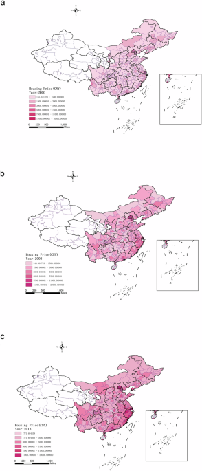
HOUSING PRICES IN PREFECTURE-LEVEL CITIES This part uses ArcGIS 10.8 software and applies the natural break method to classify the housing prices of each prefecture-level city from low to

high into six levels, and specifically analyzes the spatial and temporal evolution characteristics of China’s housing prices (Balsa-Barreiro et al., (2019)). Due to space limitations, Fig. 1

only provides the spatial distribution of house prices in 2000, 2008, and 2013. It can be seen from Fig. 1 that the housing prices in China’s prefecture-level cities have generally been on

the rise. In 2000, most prefecture-level city house prices were in the first and second levels; by 2008, many prefecture-level city house prices had jumped to the third or fourth levels; and

by 2013, housing prices in eastern coastal cities had reached the fifth and sixth levels. At the same time, the housing prices of prefecture-level cities show obvious spatial heterogeneity.

This is mainly reflected in the fact that housing prices in eastern coastal cities are higher than those in central and western inland cities; the housing prices of core cities and

surrounding cities within a province are generally higher than those of cities in provincial border areas. Taking the housing prices of prefecture-level cities in Zhejiang Province and

neighboring provinces in 2013 as an example, it can be clearly seen that the housing prices of prefecture-level cities in Zhejiang Province had reached the fourth level or above, while those

in the border areas of neighboring provinces were at least one level lower, especially in inland provinces. SPATIAL WEIGHTING MATRIX AND SPATIAL CORRELATION TEST OF HOUSING PRICES IN

PREFECTURE-LEVEL CITIES SPATIAL WEIGHTING MATRIX In spatial econometrics, the quality of the empirical tests is often influenced by the selection of the spatial weighting matrix. Anselin

(1988) provided three common criteria for constructing the spatial weighting matrix: the spatial distance criterion, the geographic proximity criterion, and the K-order proximity criterion.

In this paper, the geographic proximity criterion is used to construct a spatial proximity weighting matrix to reflect the spatial correlation among prefecture-level cities. There are two

reasons for this: first, the provinces in eastern China are economically developed and densely populated but relatively small in area, while the western provinces are economically

underdeveloped and less densely populated but vast in area, thus the spatial weighting matrix of Chinese provinces constructed using the spatial distance criterion and the K-order proximity

criterion is unreliable (Gao and Hua, 2012). Second, this paper needs to identify whether there is a significant difference in the degree of spatial correlation between house prices of

prefecture-level cities within and between provinces, and the geographic proximity weighting matrix constructed based on the geographic proximity criterion can visualize the influence of

provincial administrative boundaries. The spatial proximity weighting matrix \(W,\) \({W}_{1}\) and \({W}_{2}\) are set as follows:

$$\begin{array}{ll}\quad{w}_{ij}=\left\{\begin{array}{l}1\,{\rm{Spatial}}\,{\rm{proximity}}\\ 0\qquad\quad{\rm{others}}\end{array}\right.\\

{w}_{1,i,j}=\left\{\begin{array}{l}1\,{\rm{intra}}-{\rm{provincial}}\,{\rm{spatial}}\,{\rm{proximity}}\\ 0\qquad\quad{\rm{others}}\end{array}\right.\\

{w}_{2,i,j}=\left\{\begin{array}{l}1\,{\rm{Inter}}-{\rm{provincial}}\,{\rm{spatial}}\,{\rm{proximity}}\\ 0\qquad\quad{\rm{others}}\end{array}\right.\end{array}$$ (3) where, \({w}_{{ij}}\) is

the element in spatial proximity weighting matrix \(W\), \({w}_{1,i,j}\) is the element in intra-provincial spatial proximity weighting matrix \({W}_{1}\), and \({w}_{2,i,j}\) is the

element in inter-provincial spatial proximity weighting matrix \({W}_{2}.\,\)Obviously,\(\,W\) is equal to \({W}_{1}\) plus \({W}_{2}\)Footnote 8. The intra-provincial and inter-provincial

spatial proximity of prefecture-level cities is shown in Fig. 2 (Balsa-Barreiro et al., (2022)). SPATIAL CORRELATION TEST First, the scatter plots of house prices in prefecture-level cities

compared to those in intra-provincial or inter-provincial neighboring prefecture-level cities, as shown in Fig. 3, indicate a significant positive correlation between house prices in

prefecture-level cities, not only with those in intra-provincial neighboring prefecture-level cities (the left side of Fig. 3) but also with those in inter-provincial neighboring

prefecture-level cities (the right side of Fig. 3). Further comparison of the left side of Fig. 3 and the right side of Fig. 3 reveals a difference in the degree of correlation between house

prices in prefecture-level cities and those in adjacent prefecture-level cities within and between provinces. Furthermore, the Moran’s I statistics of house prices in prefecture-level

cities and house prices in provincial and inter-provincial neighboring prefecture-level cities, as shown in Table 2, indicate a significant spatial correlation between house prices in

prefecture-level cities and those in provincial and inter-provincial neighboring prefecture-level cities, as suggested by Moran’s I values significant at the 1% level (except for the value

for inter-provincial neighboring cities in 2004). Additionally, there is a significant difference between these two spatial correlations, with the Moran’s I values differing by an average of

more than 34%Footnote 9. The above results initially suggest that the house prices of neighboring prefecture-level cities have an important impact on the house prices of the local city.

Moreover, this impact varies depending on interprovincial administrative boundaries. Therefore, it is necessary to consider not only the impact of house prices in neighboring

prefecture-level cities but also the differences between intra-provincial and inter-provincial proximity. BASELINE RESULTS Table 3 reports the estimated results of the panel data model

(pooled regression model, fixed effect, and random effect) without considering spatial correlation. The Hausman Test statistic is 263.446 and significant at the 1% level, indicating that the

fixed effects model (FE) is more appropriate than the random effects model (RE). The maximum likelihood value suggests that the fixed effects model (FE) is also more suitable than the

pooled regression model (Pooled OLS). However, both the LM spatial error test and the LM spatial lag test reject the assumption that there is no spatial correlation at the 1% significance

level, further suggesting the need to consider spatial correlation among house prices at the prefecture level in the empirical analysis. Therefore, spatial econometric models under fixed

effects are used thereafter. Table 4 presents the results of the panel data model under various spatial correlations, namely the spatial lag model (SAR), the spatial Durbin model (SDM), the

spatial error model (SEM), and the extended spatial Durbin model (ESDM). As shown in Table 4, the sign and significance of the main explanatory variables are consistent across all models.

The following main conclusions can be drawn based on the results in Table 4. First, the ESDM is the optimal model for studying the problem in this paper. On the one hand, the LR spatial

error test statistic (137.114) and the Wald spatial error test statistic (136.680) both reject the null hypothesis at the 1% significance level, indicating that the SDM is more suitable than

the SEM. Similarly, the LR spatial lag test statistic (150.519) and the Wald spatial lag test statistic (164.742) both reject the null hypothesis, indicating that the SDM is more suitable

than the SAR. On the other hand, the difference between the estimated coefficients \(({\varphi }_{1}-{\varphi }_{2})\) of the intra-provincial spatial proximity term and inter-provincial

spatial proximity term is significantly non-zero at the 1% significance levelFootnote 10, indicating that there is a significant difference in the spatial correlation between

prefecture-level city house prices within and between provinces, and the ESDM is more appropriate compared to the SDM. Finally, the maximum log-likelihood value of the ESDM (672.38) is

larger than that of the SDM (653.921) and is the maximum among all models. Therefore, in the subsequent analysis, this paper adopts the estimation results of the ESDM (column 4)Footnote 11.

Second, there is spatial correlation of house prices between neighboring prefecture-level cities, and housing possesses both consumption and investment attributes. In the ESDM (column 4),

the estimated coefficients of the intra-provincial spatial proximity term and the inter-provincial spatial proximity term are 0.285 and 0.108, respectively, and both are significant at the

1% level. This indicates that a 1% increase in house prices of neighboring prefecture-level cities within a province leads to a 0.285% increase in house prices of local prefecture-level

cities, while a 1% increase in house prices of neighboring prefecture-level cities between provinces leads to a 0.108% increase in house prices of local prefecture-level cities. In other

words, the increase in house prices in a prefecture-level city drives the increase in house prices in adjacent prefecture-level cities, and the spatial correlation of house prices among

prefecture-level cities is significant (Wang, 2012; Ding and Ni, 2015). According to mechanisms 1–3, it is known that the mechanisms of population, capital, and information are all reasons

for the spatial correlation of house prices. In addition, the economic and non-economic factors, such as housing completion area and loans from financial institutions, are all significant,

which also indicates that housing has both consumption and investment attributes during the sample periodFootnote 12. Third, interprovincial administrative boundaries have a shielding effect

on the interprovincial linkage of house prices in prefecture-level cities, and housing is still dominated by consumption attributes and complemented by investment attributes. In the ESDM,

the effect of interprovincial administrative boundaries on house prices of prefecture-level cities is captured by the difference between the coefficients \(({\varphi }_{1}-{\varphi }_{2})\)

of the interaction term of the intra-provincial proximity matrix with house prices and the interaction term of the inter-provincial proximity matrix with house prices. In column (4), the

difference between the above two coefficients is 0.177 and is significant at the 1% level, which indicates that inter-provincial administrative boundaries lower the strength of spatial

correlation of house prices between inter-provincial prefecture-level cities by 62.11%Footnote 13. These results illustrate that although housing has both consumption and investment

attributes, it is dominated by consumption attribute and supplemented by investment attribute. The explanation is that under the regional cultural differences and the hierarchical management

system, the migration of population mainly occurs between cities within the province, and thus the spatial correlation of house prices between prefecture-level cities within the province is

much higher than that between provinces. Data from the sixth national population census shows that between 2000 and 2010, the share of urban and town residents moving within the province

accounted for 87% and 77% of the total mobile population, respectively (Xu S et al. 2016). SPATIAL CORRELATION OF HOUSE PRICES BEFORE AND AFTER THE SUBPRIME CRISIS In 2007, the subprime

mortgage crisis in the US led directly to a sudden fall in China’s house prices in 2008 (as shown in Fig. 1). However, at the start of 2009, house prices resumed a full-scale surge. This

section identifies the housing attributes in China before and after the crisis. Table 5 presents the sub-sample regression results from 2000 to 2008 and 2009 to 2013Footnote 14. The

following findings can be obtained from Table 5. First, before 2008, housing was dominated by consumption attribute. During 2000–2008, the estimated coefficient (\({\varphi }_{1}\)) of the

intra-provincial spatial proximity term is 0.221 and is significant at the 1% level, but the coefficient (\({\varphi }_{2}\)) of the inter-provincial spatial proximity term is insignificant.

The difference between the two coefficients (\({\varphi }_{1}-{\varphi }_{2}\)) is 0.153 and is significant at the 5% level, suggesting that before the crisis, there were significant

differences in the spatial correlation of house prices between prefecture-level cities within and between provinces, and the spatial correlation occurred mainly between cities within

provinces. This result illustrates that before the crisis, housing was dominated by consumption attribute in China. In the context of intra-provincial mobility of urban residents (Xu S et

al. 2016), it is the consumption attribute of housing that makes the spatial linkage of house prices in prefecture-level cities insignificant between provinces. This further explains that

the rise in house prices before the crisis was mainly caused by the release of rigid demand. In 1998, the per capita residential area of urban residents was only 18.66 m2, and by 2008 this

rose to 30.60 m2Footnote 15. Moreover, the significant impact of economic factors such as disposable per capita income and housing completion area also indicates that China’s housing was

dominated by consumption attribute before the crisis. Second, after 2008, housing became dominated by the investment attribute. The estimated coefficients of the intra-provincial spatial

proximity term and the inter-provincial spatial proximity term in 2009 to 2013 are found to be 0.318 and 0.227, both significant at the 1% level. However, the difference between the two

coefficients is no longer significant, suggesting that the spatial linkage of house prices is significant in the post-crisis period both within and between provinces, and there is no

significant difference between the two. This result implies that China’s housing has shifted to being dominated by the investment attribute in the post-crisis period. Under the investment

attribute, it is the capital and information mechanisms that lead to no difference in the intra- and inter-provincial linkage of house prices. After a short decline in 2008, the average

sales price of commercial housing and residential housing in China rose by 21.05% and 25.57%, respectively, in 2009Footnote 16. Meanwhile, the housing vacancy rate soared from below 5.00%

prior to 2007 to 6.49% in 2009. All of this indicates a change in the dominant attribute of housing in China. ROBUSTNESS TEST The causes of the differences in the spatial correlation of

house prices before and after the subprime crisis could be either institutional changes that have led to a decline in the influence of inter-provincial administrative boundaries or changes

in the dominant attribute of housing, which need to be identified. This section examines the differences in the impact of inter-provincial administrative boundaries on the spatial spillover

of economic growth by comparing the shielding effect before and after the subprime crisis, thus conducting a robustness test of the findings in Section 5. In fact, the subprime crisis in the

US in 2007 not only led to the fall in China’s house prices in 2008, but also a decline in China’s economy from May 2008 (Jin, 2010; Zhang, 2018). Therefore, the results of the sub-sample

estimates of economic growth for the periods 2000–2008 and 2009–2013 are comparable. Table 6 reports the results of the ESDM of economic growth rates before and after the subprime crisis. As

can be seen from Table 6, the spatial spillover effect of economic growth became weaker after 2008, but the shielding effect of inter-provincial administrative boundaries on the spatial

spillover of economic growth increased. Before and after the subprime crisis, the spatial spillover effect of the economic growth rate of neighboring prefectures within the province

decreased from 0.459 to 0.290, and the spatial spillover effect of the economic growth rate of neighboring prefectures between provinces decreased from 0.200 to 0.109 (insignificant), while

the shielding degree of the inter-provincial administrative boundary increased from 56.33% to 62.41%Footnote 17. This indicates that the shielding effect of inter-provincial administrative

boundaries on the spatial spillover of economic growth became stronger after the outbreak of the subprime crisis. This further implies that, in the post-crisis period, the substantial

increase in the spatial correlation of house prices in inter-provincial prefectures was not caused by regional culture and economic institutional changes but by the shift in the dominant

attribute of Chinese housing. Thus, this serves as supporting evidence for the robustness of the conclusions in Section 5. CONCLUSIONS AND IMPLICATIONS In recent years, the Chinese

government has repeatedly stressed the need to adhere to the principle that ‘houses are for living, not for speculation’. In this context, identifying the attributes of housing is the

prerequisite for formulating and implementing long-term housing management policies. This paper first explores the heterogeneity of the spatial correlation of house prices based on the

mechanism of spatial correlation and then empirically tests the heterogeneous spatial correlation of house prices among prefecture-level cities using the extended spatial Durbin model to

identify the dominant attribute of housing in different periods, finally conducting robustness tests using economic growth data. The results of the study suggest that housing has both

consumption and investment attributes, with the consumption attribute dominating and the investment attribute supplementing. There is a spatial correlation of house prices between

neighboring prefecture-level cities, and inter-provincial administrative boundaries have a shielding effect on the cross-provincial spatial correlations of house prices. A 1% increase in

house prices of neighboring prefecture-level cities within a province leads to a 0.285% increase in house prices of local prefecture-level cities, while a 1% increase in house prices of

neighboring prefecture-level cities between provinces leads to a 0.108% increase in house prices of local prefecture-level cities. This implies that the inter-provincial administrative

boundaries lower the spatial correlation of house prices between prefecture-level cities by 62.11%. Further research shows that before 2008, housing was dominated by the consumption

attribute. The spatial correlation of house prices between prefecture-level cities varied significantly within and between provinces, with the spatial correlation primarily occurring between

cities within the same province. After 2008, housing became dominated by the investment attribute. The spatial correlation of house prices between prefecture-level cities became significant

both within and between provinces, with no significant difference between them, indicating that the dominant attribute of housing had shifted from consumption to investment after 2008.

According to the findings of this paper, adhering to the principle of ‘housing without speculation’ requires weakening the investment attribute of housing by raising arbitrage costs and

stabilizing residents’ expectations. The government can raise the cost of arbitrage by imposing a housing tax, extending the holding period after housing transactions, raising mortgage rates

for multiple properties, and strictly controlling the scale of real estate financing. Most of these policies have already been introduced or implemented, such as the housing tax pilot in

Shanghai and Chongqing. The CBRC issued the Notice on the Special Inspection of Real Estate Business of Banking Institutions in 2019. In addition, the government can stabilize residents’

expectations by controlling housing prices and adjusting the housing market structure. First, efforts should be made to resolutely curb the continuous and rapid rise in housing prices and to

establish expectations for the stable development of the housing market. Second, increasing the supply of housing and developing the rental market can help avoid panic buying. Although this

paper innovatively identifies the stage attributes of real estate based on spatial correlation differences in housing prices within and between provinces, there are still some deficiencies

in the following aspects. First, China has a vast territory, and there is a large gap in area and economic development between provinces. It is likely that the spatial correlation will not

be the same for all neighboring provinces (and possibly not even within different provinces). However, based on the identification strategy of whether there is an inter-provincial proximity

relationship, it is difficult to reflect the spatial correlation differences in housing prices between different provinces. In the future, further research will be conducted on the impact of

provinces’ ‘border situations’ and ‘border areas’ on housing prices. Second, it is difficult to analyze heterogeneity by region. In the process of sub-regional discussion, the deletion of

some provincial samples makes the spatial proximity matrix meaningless. For example, in the discussion of the eastern, central and western regions, Nanjing in the eastern region originally

borders Chuzhou, Ma’anshan and Xuancheng in the central region. However, in the subsample regression of eastern cities, it is set to not border on provincial cities. Third, due to sample

data limitations, this paper fails to identify the dominant attributes of housing prices in recent years. Since the China Regional Economic Statistical Yearbook is only publicly available up

to 2014, and the Urban Statistical Yearbook does not include data from ‘autonomous prefectures’ and ‘leagues’ such as Xiangxi Tujia-Miao Autonomous Prefecture or Xing’an League, it can only

identify the dominant attributes of China’s housing prices before 2013. However, this does not affect the innovation of the test strategy or the identification of attributes between

samples. DATA AVAILABILITY All data generated or analyzed during this study are included in this published article. NOTES * Theoretically, the border effect has given rise to the

‘international trade puzzle’ and the ‘law of one price paradox’. Empirically, it has been measured mainly from the perspectives of trade flow differences and price index differences. *

Specifically, 63% of the respondents believe that the local government requires enterprises to recruit workers to give priority to local household registration, 62% believe that the cost of

local schooling for children of non-local staff is too high, 57% believe that it is difficult for non-local staff to settle down in the local area and solve the household registration, 56%

believe that it is difficult to provide pension, medical and unemployment insurance for non-local staff because of the imperfect functions of the government, and 55% believe that there are

local protection methods that restrict the flow of technical personnel, especially important technical personnel. * Of course, real estate regulation policies such as purchase restrictions

on purchases and loans have weaken the mechanism of capital flow in real estate market, but not affected the spatial correlation of urban house prices formed under the mechanism of capital

flow. Therefore, there is no specific analysis of the impact of real estate regulation policies. * There are two reasons for excluding the data of Xinjiang, Tibet, Qinghai and Gansu

provinces or autonomous regions. Firstly, there are many prefecture-level cities in these four provinces or autonomous regions whose data are missing. Secondly, during 2000-2003, there were

many cases of withdrawal and merger of counties and cities. * To ensure comparability of data, through county-level data information, Zhongning County was removed from Wuzhong City and

Haiyuan County and the former Zhongwei County were removed from Guyuan City in 2003 and earlier data (on 6 February 2004, the Notice of ‘the People’s Government of Ningxia Hui Autonomous

Region on the Abolition of Zhongwei County and the Establishment of Prefectural-level Zhongwei City’ established prefecture-level Zhongwei City, including Zhongning County, Haiyuan County

and the former Zhongwei County, which were transferred from Wuzhong and Guyuan City). * To ensure comparability of data, through county-level data, lujiang County of Chaohu City was merged

into Hefei city, Hanshan County and Hexian County were merged into Maanshan City, and Wuwei County was merged into Wuhu City respectively in 2011 and later data (on 14 July 2011, the ‘Reply

on the Approval of the Abolition of the Prefectural-level Chaohu City and the Adjustment of Some Administrative Divisions in Anhui Province’ split the prefectural-level Chaohu City into

three, which were subsumed into Hefei, Wuhu and Maanshan). * The price index data of some prefecture-level cities over the years is missing. For example, the Tibetan Statistical Yearbook did

not publish the price index of all prefecture-level cities before 2010, the Hunan Statistical Yearbook did not publish the price index of prefecture-level cities after 2006 and published

the price index of 14 surveyed cities and counties from 2002 to 2006. Therefore, provincial-level data were uniformly used to make adjustments. * In practice, each row in \(W\) is first

normalized to 1 by equation \({w}_{i,j}=\frac{{w}_{i,j}}{{\sum }_{j}{w}_{i,j}}\); Then, in the standardized \(W\), if the prefecture-level cities belong to different provinces, the

corresponding elements are all 0 to obtain the intra-provincial neighborhood spatial weighting matrix \({W}_{1}\). If the prefecture-level cities belong to the same province, the

corresponding elements are all 0 to obtain the inter-provincial neighborhood spatial weighting matrix \({W}_{2}\). * 34% is obtained by dividing the difference between the Moran’I values of

the intra-provincial neighborhood and inter-provincial neighborhood by the Moran’I values of the intra-provincial neighborhood, averaging them and multiplying by 100%. * At present, there

are no mature test statistics to compare the ESDM with the SDM. * It is worth noting that the spatial correlation of house prices between prefecture A and prefecture B is a reciprocal

concept, so there is no need to consider the estimation bias caused by reverse causality in the model; In addition, in the spatial econometric model, when the omitted variable has spatial

dependence with the existing explanatory variable, and the perturbation term has spatial dependence as in the SEM, the coefficient estimation of the spatial correlation term of the explained

variable is consistent, Therefore, the estimation results of core explanatory variables can not be affected even if there are missing variables in the model. So, the estimation results

based on the ESDM are reliable. * At this point, the coefficient on urban per-capita disposable income is no longer significant, most likely because Chinese residents tend to buy homes on a

household basis, it is common for two or three generations to buy houses together. Thus, household wealth may be a better proxy for purchasing power, but data on household wealth at the

prefectural level could not be found, so no comparative analysis has been undertaken here. * The specific calculation process is as follows: \(\,(\varphi 1\,-\,\varphi 2)/\,\varphi 1* 100 \%

=(0.285-0.108)/0.285* 100 \% =62.11 \%\) * In the sub-sample regression results for 2000–2007 and 2010–2013, the estimates of \({\varphi }_{1}\) are 0.218 and 0.310, the estimates of

\({\varphi }_{2}\) are 0.051 and 0.307, and the estimates of \(({\varphi }_{1}-{\varphi }_{2})\) are 0.166 and 0.003, respectively. In other words, compared with the results of 2000–2008,

the inter-provincial administrative boundary had a stronger shielding effect on the inter-provincial linkage of house prices during 2000–2007 than the period of 2000–2008, and the

consumption attribute of real estate was more dominant; Compared with the results of 2009–2013, while the intra-provincial linkage of house prices during 2010–2013 was more like the

inter-provincial linkage than 2009–2013. Due to the length of the paper, the specific regression results from 2000 to 2007 and 2010 to 2013 are not given. Interested readers can contact the

author for them. * Based on data from national statistics bureau and relevant public information. * Data from Zhang Chuanchuan et al. (2016). * The specific calculation process is as

follows: \((0.458-0.200)/0.458* 100 \% =56.33 \%\); \((0.290-0.109)/0.290* 100 \% =62.41 \%\). REFERENCES * Akerlof G (1997) Social distance and social decisions. Econometrica

65(5):1005–1028 Article  MathSciNet  MATH  Google Scholar  * Anderson JE, Van Wincoop E (2003) Gravity with gravitas: a solution to the border puzzle. Am Econ Rev 93(1):170–192 Article  MATH

  Google Scholar  * Anselin L (1988) Spatial econometrics: methods and models. Springer, Netherlands Book  MATH  Google Scholar  * Balsa-Barreiro J, Li Y, Morales A, Pentland (2019)

Globalization and the shifting centers of gravity of world’s human dynamics: Implications for sustainability. J Clean Prod 239:117923 Article  Google Scholar  * Balsa-Barreiro J, Menendez M,

Morales AJ (2022) Scale, context, and heterogeneity: the complexity of the social space. Sci Rep 12(1):9037 Article  ADS  CAS  PubMed  PubMed Central  MATH  Google Scholar  * Black A,

Fraser P, Hoesli M (2006) House prices, fundamentals, and bubbles. J Bus Financ Account 10:1535–1555 Article  MATH  Google Scholar  * Brady R (2011) Measuring the diffusion of housing prices

across space and over time. J Appl Econ 26(2):213–231 Article  MathSciNet  MATH  Google Scholar  * Case K, Shiller R (2003) Is there a bubble in the Housing Market? Brook Pap Econ Act

2003(2):299–363 Article  MATH  Google Scholar  * Chen B, Huang S, Ouyang (2018) Can housing price drive economic growth? China Econ. Q 03:1079–1102 MATH  Google Scholar  * Deng G, Gan L, Wu

(2010) Is there an ‘Overreaction’ in the Housing Market? Manag World (06): 41–49+55 * Ding R, Ni P (2015) Regional spatial linkage and spillovers effect of house prices of China’s

cities—Based on the Panel Date of 285 cities from 2005 to 2012. Financ Trade Econ 403(6):136–150 Google Scholar  * Elhorst JP, Fréret S (2009) Evidence of political yardstick competition in

France using a two-regime spatial durbin model with fixed effects. J Reg Sci 49(5):931–951 Article  MATH  Google Scholar  * Elhorst JP (2014) Spatial econometrics: from cross-sectional data

to spatial panels. Springer, Netherlands Book  MATH  Google Scholar  * Engel C, Rogers JH (1996) How wide is the border? Am Econ Rev 86(5):1112–1125 MATH  Google Scholar  * Fan Z, Zhang H,

Chen J (2018) The spillover effects and siphon effects of public transportation on housing. China Industrial Econ 35(5):99–117 MATH  Google Scholar  * Goodman AC, Thibodeau TG (2008) Where

are the speculative bubbles in US housing markets? J Hous Econ 17(2):117–137 Article  MATH  Google Scholar  * Green R (1999) Land use regulation and the price of housing in a suburban

Wisconsin County. J Hous Econ 8(2):144–159 Article  MATH  Google Scholar  * Gao J (2015) Current situation analysis and prospect of housing market. China Dev Obs 122(2):48–54 MATH  Google

Scholar  * Gao X, Long X (2016) Does cultural segmentation caused by administrative division harm regional economic development in China? China Econ Q 15(2):647–674 MATH  Google Scholar  *

Gao Y, Hua Y (2012) Spatial econometric empirical analysis of heterogeneous human capital’s effect on economic growth. Econ Sci 187(1):39–50 MathSciNet  MATH  Google Scholar  * Gong R (2012)

Tax System Reform, Land Finance and House Price Levels. World Econ Pap 209(4):90–104 MATH  Google Scholar  * Gorodnichenko Y, Tesar LL (2009) Border effect or country effect? Seattle may

not be so far from Vancouver after all. Am Econ J Macroecon 1(1):219–241 Article  Google Scholar  * Gupta R, Miller SM (2012) The time-series properties of house prices: a case study of the

Southern California Market. J Real Estate Financ Econ 44(3):339–361 Article  MATH  Google Scholar  * Han L (2010) The effects of price risk on housing demand: empirical evidence from US

markets. Rev Financ Stud 23(11):3889–3928 Article  MATH  Google Scholar  * Henderson JV, Ioannides YM (1983) A model of housing tenure choice. Am Econ Rev 73(1):98–113 MATH  Google Scholar 

* He B, Yang W (2016) The diffusion of house price bubble: a new perspective of real estate market control. China Econ Stud 1:96–109 MATH  Google Scholar  * He X, Tian L, Chu E (2017) The

spatial heterogeneity of house price volatility in China from the perspective of migration. Popul Econ 225(6):43–57 MATH  Google Scholar  * He X, Fei H, Zhang Y (2015) A study on the

risk-return relationship for housing: evidence from housing consumption Hedge Effect. J Financ Res 416(2):76–94 MATH  Google Scholar  * Holly S, Hashem Pesaran M, Yamagata T (2011) The

spatial and temporal diffusion of house prices in the UK. J Urban Econ 69(1):2–23 Article  MATH  Google Scholar  * Holmes M, Grimes A (2008) Is there long-run convergence among regional

house prices in the UK? Urban Stud 45(8):15–31 Article  MATH  Google Scholar  * Hughes G, McCormick B (1994) Did migration in the 1980s narrow the North-South divide? Economica

61(244):509–527 Article  MATH  Google Scholar  * Huang F, Zhou J, Li Z, Hou T (2009) Relationships effect among housing prices of chinese big cities based on cointegration and vector error

correction model. Q J Manag 4(2):122–143 MATH  Google Scholar  * Huang X, Dong X, Ping X (2018) Policy evaluation of local government real estate market regulation based on restriction of

purchase, loan and sale. Reform 291(5):107–118 MATH  Google Scholar  * Jarociński M, Smets FR (2008) ‘House Prices and the Stance of Monetary Policy’. Fed Reserve Bank St Louis Rev

90(4):339–365 MATH  Google Scholar  * Jia C, Ge Y (2015) Urban administrative level, resource aggregation capacity and house price level differences. Research on Financ Econ Issues

383(10):131–137 MATH  Google Scholar  * Jin B (2010) China’s Industry under the Global Financial Crisis. China Industrial Econ 268(7):5–13 MATH  Google Scholar  * Ke S, Huang J (2012)

Research on the herd behavior of Chinese real estate market based on non-linear test model CSAD. Manag Rev 24(9):19–25+74 MATH  Google Scholar  * Kuang W (2005) A Study on the relationship

between housing pricing and land pricing: basic model and evidence from China. Financ Trade Econ (11): 58–65+107 * Kuang W (2010) Expectation, speculation and urban housing price volatility

in China. Econ Res J 45(9):67–78 MATH  Google Scholar  * Li J, You W, Sun P (2017) Do migrants boost city’s housing price? An empirical study based on China’s city data. Nankai Econ Stud

193(1):58–76 MATH  Google Scholar  * Li Z, Lin J, Deng H (2021) Beyond cultural barriers in interprovincial migration: information communication and identity recognition. China Econ Q

21(5):1691–1710 MATH  Google Scholar  * Li Z, Yu S, Zheng J (2016) Real state attributes, income gap and change trend of housing prices. J Financ Econ 42(7):122–133 CAS  MATH  Google Scholar

  * Liang Y, Gao T (2007) Empirical analysis on real estate price fluctuation in different provinces of China. Econ Res J (8):133–142 * Liang Y, Gao T (2006) Empirical analysis on the causes

of commodity residential sales price fluctuations in China. Manag World (8):76–82 * Lin J, Zhou S, Wei W (2012) Prices of urban real estate, housing property and subjective well-being.

Financ Trade Econ 366(5):114–120 MATH  Google Scholar  * Liu C, Han W, Li M (2014) Multiple price ranges and choice behaviors of buyers: the causes of the rising price of housing. Econ Rev

188(4):96–107 MATH  Google Scholar  * Lu M, Ou H, Chen B (2014) Rationality or bubble: empirical research on urbanization, migration and house prices. J World Econ 425(1):30–54 MATH  Google

Scholar  * Lv J (2010) The measurement of the bubble of urban housing market in China. Econ Res J 45(6):28–41 MATH  Google Scholar  * Lv L, Liu H (2019) Research on the measurement, network

structure and influencing factors of the spillover effect of urban housing prices. Econ Rev 216(2):125–139 MATH  Google Scholar  * McCallum J (1995) National Borders Matter: Canada-US

regional trade patterns. Am Econ Rev 85(3):615–623 MATH  Google Scholar  * Meen G (1999) Regional house prices and the ripple effect: a new interpretation. Hous Stud 14(6):733–753 Article 

MATH  Google Scholar  * Meen G (1996) Spatial aggregation, spatial dependence and predictability in the UK housing market. Hous Stud 11(3):345–372 Article  MATH  Google Scholar  * Muellbauer

J, Murphy A (1997) Booms and busts in the UK housing market. Econ J 107:1701–1727 Article  MATH  Google Scholar  * Nitsch V (2000) National borders and international trade: evidence from

the European Union. Can J Econ 33(4):1091–1105 Article  MATH  Google Scholar  * Parsley DC, Wei SJ (2001) Explaining the border effect: the role of exchange rate variability, shipping costs,

and geography. J Int Econ 55(1):87–105 Article  MATH  Google Scholar  * Raymond T (1988) Housing price, land supply and revenue from land sales. Urban Stud 35(8):1377–l392 MATH  Google

Scholar  * Sebastien B (2010) Consumption and Investment of Housing in Portfolio. Doctoral Thesis, UC Berkerley * Shiller RJ (1990) Speculative prices and popular models. J Econ Perspect

4(2):55–65 Article  MATH  Google Scholar  * Shen Y, Liu H (2004) Housing prices and economic fundamentals: a cross city analysis of China for 1995–2002. Econ Res J (6):78–86 * Sirmans GS,

Macpherson DA, Zietz EN (2005) The composition of hedonic pricing models. J Real Estate Lit 13(1):3–43 MATH  Google Scholar  * Takáts E (2012) Aging and house prices. J Hous Econ

21(2):131–141 Article  MATH  Google Scholar  * Tang W (2019) Decentralization, externalities and boundary effects. Econ Res 54(03):103–118 MATH  Google Scholar  * Tang Y, Ma C (2017) Fiscal

pressure, land finance and house price ratchet effect. Financ Trade Econ 38(11):39–54+161 MATH  Google Scholar  * Taylor JE (1986) Differential migration, networks, information and risk. Res

Hum Cap Dev (4): 147–171 * Wang H (2012) Real estate price impact factors analysis based on spatial econometrics. Econ Rev 173(1):48–56 MATH  Google Scholar  * Wang J, Liu X (2014)

Residential fundamental value, bubble component and regional spillover effect. China Econ Q 13(04):1283–1302 MATH  Google Scholar  * Wang S, Yang Z, Liu H (2008) An empirical study on the

interactive relationship between housing prices in China’s regional market cities. Res Financ Econ Issues (6):122–129 * Wang W, Rong Z (2014) Housing boom and firm innovation: evidence from

industrial firms in China. China Econ Q 13(2):465–490 MathSciNet  MATH  Google Scholar  * Wang Z, Kuang Y (2019) The impact of dialect skill on the willingness of long-term residence among

floating population. Stud Labor Econ 7(4):102–120 MATH  Google Scholar  * Wei SJ (1996) Intra-national versus international trade: how stubborn are nations in global integration? No 5531,

NBER Working Papers, National Bureau of Economic Research, Inc * Xu S, Deng Y, Wang K (2016) Interprovincial migration model, spatial pattern and citizenization path of floating population

in China. Sci Geogr Sin 36(11):1637–1642 MATH  Google Scholar  * Xu T, Yao Y (2018) Urban population migration and housing price fluctuation: an empirical research based on the census data

and baidu migration data. J Jiangxi Univ Financ Econ 115(1):11–19 MATH  Google Scholar  * Xu Y, Wu LA (2019) Dynamic relationship between Chinese provincial demographic characteristics and

housing price volatility. Stat Res 36(1):28–38 MATH  Google Scholar  * Yang Z, Zhang H, Chen J (2014a) How does potential motivation for purchasing houses again affect housing wealth effect?

A micro study based on urban household survey data. J Financ Econ 40(7):54–64 MATH  Google Scholar  * Yang Z, Zhang H, Zhao L (2014b) Dual role of housing consumption and investment:

reexamine correlation of housing and consumption in urban China. Econ Res J 49(S1):55–65 MATH  Google Scholar  * Yu H (2010) Economic fundamentals or real estate policies influence house

prices in China. Financ Trade Econ 340(3):116–122 MATH  Google Scholar  * Zhang C, Jia S, Yang R (2016) Cramped housing in ‘Ghost City’: income Inequality and the real estate bubble. J World

Econ 39(02):120–141 MATH  Google Scholar  * Zhang H (2017) House is used to live, not to fry: understanding of Xi Jinping’s Core thought of real state. Shanghai J Econ 346(07):12–19+30

Google Scholar  * Zhang L, He J, Ma R (2017) Escape from Beijing, Shanghai and Guangzhou? How house prices influence labor mobility. Int Monet Rev (11):1070–1091 * Zhang L, Zhao J, Zhang Z

(2012) High cost of living is a drag on satisfaction with quality of life in cities: a survey of quality of life in 35 Chinese cities. Econ Perspect 617(07):25–34 MATH  Google Scholar  *

Zhang Y (2018) Subprime crisis, export shock and internal governance design. China Econ Q 17(1):27–44 ADS  MATH  Google Scholar  * Zhou J (2007) Real estate: attribute transmutation,

investment activities and market evolution. Financ Trade Econ (08):115-120 * Zhou J, Wu X (2009) Research on the price spillover effect of public investment on real estate market -based on

the data of 30 provinces and cities in China. World Econ Pap 188(1):15–32 MATH  Google Scholar  Download references ACKNOWLEDGEMENTS This study is funded by the National Social Science Fund

of China (NO. 23BJY245) and the General Project of the Natural Science Foundation of Hunan province, China (NO. 2023JJ30269). We would like to express our sincere gratitude to all the

researchers who contributed to the research of this paper and all funders. AUTHOR INFORMATION AUTHORS AND AFFILIATIONS * School of Business, Hunan University of Science and Technology,

Xiangtan, Hunan, China He Wang & Shujun Yang * Hunan University of Science and Technology, Research Center for Regional High-quality Development, Xiangtan, China He Wang Authors * He

Wang View author publications You can also search for this author inPubMed Google Scholar * Shujun Yang View author publications You can also search for this author inPubMed Google Scholar

CONTRIBUTIONS He Wang: Conceptualization, Data curation, Formal analysis, Funding acquisition, Methodology, Project administration, Software, Supervision, Validation, Writing – review &

editing. Shujun Yang: Conceptualization, Formal analysis, Software, Validation, Visualization, Writing – original draft. CORRESPONDING AUTHOR Correspondence to Shujun Yang. ETHICS

DECLARATIONS COMPETING INTERESTS The authors declare no competing interests. ETHICAL APPROVAL This article does not contain any studies with human participants performed by any of the

authors. INFORMED CONSENT This article does not contain any studies with human participants performed by any of the authors. ADDITIONAL INFORMATION PUBLISHER’S NOTE Springer Nature remains

neutral with regard to jurisdictional claims in published maps and institutional affiliations. SUPPLEMENTARY INFORMATION RESEARCH SAMPLE RIGHTS AND PERMISSIONS OPEN ACCESS This article is

licensed under a Creative Commons Attribution-NonCommercial-NoDerivatives 4.0 International License, which permits any non-commercial use, sharing, distribution and reproduction in any

medium or format, as long as you give appropriate credit to the original author(s) and the source, provide a link to the Creative Commons licence, and indicate if you modified the licensed

material. You do not have permission under this licence to share adapted material derived from this article or parts of it. The images or other third party material in this article are

included in the article’s Creative Commons licence, unless indicated otherwise in a credit line to the material. If material is not included in the article’s Creative Commons licence and

your intended use is not permitted by statutory regulation or exceeds the permitted use, you will need to obtain permission directly from the copyright holder. To view a copy of this

licence, visit http://creativecommons.org/licenses/by-nc-nd/4.0/. Reprints and permissions ABOUT THIS ARTICLE CITE THIS ARTICLE Wang, H., Yang, S. The influence of administrative border on

the spatial correlation of house prices: evidence from China. _Humanit Soc Sci Commun_ 12, 248 (2025). https://doi.org/10.1057/s41599-025-04463-1 Download citation * Received: 27 May 2024 *

Accepted: 28 January 2025 * Published: 24 February 2025 * DOI: https://doi.org/10.1057/s41599-025-04463-1 SHARE THIS ARTICLE Anyone you share the following link with will be able to read

this content: Get shareable link Sorry, a shareable link is not currently available for this article. Copy to clipboard Provided by the Springer Nature SharedIt content-sharing initiative