Exploring the limits of community detection strategies in complex networks

ABSTRACT The characterization of network community structure has profound implications in several scientific areas. Therefore, testing the algorithms developed to establish the optimal

division of a network into communities is a fundamental problem in the field. We performed here a highly detailed evaluation of community detection algorithms, which has two main novelties:

1) using complex closed benchmarks, which provide precise ways to assess whether the solutions generated by the algorithms are optimal; and, 2) A novel type of analysis, based on

hierarchically clustering the solutions suggested by multiple community detection algorithms, which allows to easily visualize how different are those solutions. Surprise, a global parameter

that evaluates the quality of a partition, confirms the power of these analyses. We show that none of the community detection algorithms tested provide consistently optimal results in all

networks and that Surprise maximization, obtained by combining multiple algorithms, obtains quasi-optimal performances in these difficult benchmarks. SIMILAR CONTENT BEING VIEWED BY OTHERS

LOCAL DOMINANCE UNVEILS CLUSTERS IN NETWORKS Article Open access 31 May 2024 REPRESENTATIVE COMMUNITY DIVISIONS OF NETWORKS Article Open access 17 February 2022 TWO ANTAGONISTIC OBJECTIVES

FOR ONE MULTI-SCALE GRAPH CLUSTERING FRAMEWORK Article Open access 18 April 2025 INTRODUCTION Complex networks are widely used for modeling real-world systems in very diverse areas, such as

sociology, biology and physics1,2. It often occurs that nodes in these networks are arranged in tightly knit groups, which are called communities. Knowing the community structure of a

network provides not only information about its global features, i.e., the natural groups in which it can be divided, but may also contribute to our understanding of each particular node in

the network, because nodes in a given community generally share attributes or properties3. For these reasons, characterizing which are the best strategies to establish the community

structure of complex networks is a fundamental scientific problem. Many community detection algorithms have been proposed so far. The best way to sort out their relative performances is by

determining how they behave in standard synthetic benchmarks, consisting of complex networks of known structure. There are two basic types of benchmarks, which we have respectively called

_open_ and _closed_4,5,6. Open benchmarks use networks with a community structure defined _a priori_, which is progressively degraded by randomly rewiring links in such a way that the number

of connections among nodes in different communities increases and the network evolves toward an unknown, “open-ended” structure5,6,7,8,9,10,11. In open benchmarks, the performance of an

algorithm can be measured by comparing the partitions that it obtains with the known, initial community structure, being increasingly difficult to recover that structure as the rewiring

progresses. The first commonly used open benchmark was developed by Girvan and Newman (GN benchmark)12. It is based on a network with 128 nodes, each with an average number of 16 links,

split into four equal-sized communities. It is however well established that the GN benchmark is too simple. Most algorithms are able to provide good results when confronted with it7,8.

Also, the fact that all communities are identical in size makes some algorithms that favor erroneous structures (e.g., those unable to detect communities that are small relative to the size

of the network6,7,8,13,14,15) to perform artificially well in this benchmark. These results indicated the need to develop more complex benchmarks. A new type was suggested by Lancichinetti,

Fortunato and Radicchi (LFR benchmarks), which has obvious advantages over the GN benchmark16. In the GN networks, node degrees follow a Poisson distribution. However, in many real networks

the degree distribution displays a fat tail, with a few highly connected nodes and the rest barely linked. This suggests that its distribution may be modeled according to a power law. In the

LFR benchmarks, both the degrees of the nodes and the community sizes in the initial networks can be adjusted to follow power laws, with exponents chosen by the user. In this way, realistic

networks with many communities can be built. LFR benchmarks are much more difficult than GN benchmarks, with many algorithms performing poorly in them6,8,9,10,11. Notwithstanding these

advantages, typical LFR benchmarks are based on networks where all communities have similar sizes4,5,6,8. This led to the proposal of a third type of benchmark, based on Relaxed Caveman (RC)

structures17. In this type of benchmarks, the initial networks are formed by a set of isolated cliques, each one corresponding to a community, which are then progressively interconnected by

rewiring links. The possibility of selecting the size of each initial clique makes the RC benchmarks ideal for building highly skewed distributions of community sizes, which constitute a

stern test for most algorithms4,5,6. In open benchmarks, when the original structure is largely degraded – and especially if the networks used in the benchmark are large and have a complex

community structure – it generally happens that all algorithms suggest partitions different from the initial one. However, this can be due to two very different reasons: either the

algorithms are not performing well or all/some of them indeed are optimally recovering the community structure present in the network, but that structure does not anymore correspond to the

original one. The lack of a way to discriminate between these two potential causes is a limitation of all open benchmarks. To overcome this problem, we recently proposed a different type of

benchmark, which we called _closed_4,5. Closed benchmarks also start with a network with known community structure. However, the rewiring of the links is not random, as in open benchmarks.

It is instead guided from the initial network toward a second, final network, which has exactly the same community structure that the initial one, but with the nodes randomly reassigned

among communities. The rewiring process in these benchmarks is called _Conversion_ (C) and ranges from 0% to 100%. When C = 50%, half of the links that must be modified in the transition

from the initial to the final networks have been already rewired and C = 100% indicates that the final structure has been obtained. Further details about closed benchmarks can be found in

one of our recent papers, in which we extensively described its behavior and how they can be applied to real cases5. The main advantage of the closed benchmarks is that it is possible to

obtain quantitative information regarding whether a given partition is optimal or not, using analyses based on a parameter called Variation of Information (VI18). By definition, VI(X,Y) = H

(X) + H(Y) − 2 I(X,Y), where X and Y are the two partitions to be compared, H(X) and H(Y) are the entropies of each partition and I(X,Y) is the mutual information between X and Y. The logic

behind VI is to provide a distance measure indicating how different are two partitions once it is taken into account not only their structures but also the common features present in both of

them. A very important reason for using VI is that it is a metric18. In the context of the closed benchmarks, this means that VI satisfies the triangle inequality: VIIE + VIEF ≥ VIIF,

where: 1) VIIE is the variation of information for the comparison between the original community structure known to be present in the initial network (I) and the one deduced for an

intermediate network (E), generated at a certain point of the conversion process; 2) VIEF is obtained comparing that intermediate structure and the community structure of the final network

(F), which is also known; and, 3) VIIF is obtained when the initial and final structures are compared. Assuming that, along the conversion process, the network moves away from the initial

structure at the same rate as it approaches the final one, an algorithm that performs optimally during the whole conversion process should generate solutions satisfying the equality VIIE +

VIEF = VIIF – where E is in this context the partition proposed by the algorithm – while deviations from this equality, which can be summarized with the value VIδ = VIIF − (VIIE + VIEF),

would indicate suboptimal performance4,5. Another advantage of the closed benchmarks is that the identical community structure in the original and final networks implies a second

quantitative feature: the solutions provided by an algorithm must be symmetrical along the conversion of one into the other. For example, at C = 50%, a correct partition must be equally

similar to both the initial and final networks. Finally, it is also significant to point out that closed benchmarks are very versatile, given that any network, for example those

traditionally used in open GN, LFR or RC benchmarks, can be also analyzed in a closed configuration. All the analyses described so far, in both open and closed benchmarks, require the

community structure to be known a priori. Additional useful information may be obtained by evaluating the results of the different algorithms with measures able to establish the quality of a

partition by criteria that are independent of knowing the structures originally present in the networks. In the past, one such global measure of partition quality, called modularity19, was

extensively used. However, multiple works have shown that modularity-based evaluations are often erroneous4,6,13,14,15. In recent studies, we introduced a new global measure, called Surprise

(S), which has an excellent behavior in all networks tested4,5,6. Surprise measures the probability of finding a particular number of intracommunity links in a given partition of a network,

assuming that those links appeared randomly (see Methods for details and S formula). We have shown that S can be used to efficiently evaluate algorithms in open benchmarks and that,

according to its results in those benchmarks, the best algorithm turned out to be combining multiple methods to maximize S6. These results suggest that Surprise may also contribute to

evaluate algorithm performance in closed benchmarks and raise the question of whether S maximization could also be the best method to obtain optimal partitions in these complex benchmarks.

In this study, we carry out an extensive and detailed analysis of the behavior in closed benchmarks of a set of algorithms already used in open benchmarks in one of our recent papers6. Our

work has three well-defined sections. First, we test all those strategies in both LFR and RC closed benchmarks, being able to identify the algorithms which perform well and those that

perform poorly or are unstable. Second, we propose a novel approach to compare methods, which involves hierarchically clustering all their solutions. Applying this procedure at different

stages of the closed benchmarks, we obtain a better understanding of how the algorithms behave. Finally, we show that, as already demonstrated in open benchmarks, Surprise maximization is,

among all tested, the best strategy for community characterization in closed ones. RESULTS DETAILED BEHAVIOR OF THE ALGORITHMS The 17 algorithms tested in the LFR and RC closed benchmarks

showed very different behaviors, which are summarized in Figures 1,2,3,4. In these figures, following methods developed in previous works4,5, we show the VI values comparing the partitions

obtained by the algorithms with the known initial (red lines) and final (black lines) structures. A perfect agreement with any of these structures corresponds to VI = 0. Also, the value

(VIIE + VIEF)/2, (where E is the partition suggested by the algorithm, while I and F are, respectively, the initial and final partitions) is indicated with a blue line. As we discussed

before, if the performance of an algorithm is optimal, then, we would expect VIIE + VIEF = VIIF. This means that, in these representations, the blue line should, in the best case, be

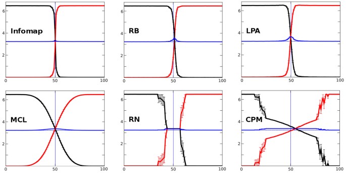
perfectly straight and located just on top of a thin dotted line also included in these figures, which corresponds to the value VIIF/2. Figure 1 shows the behavior of the six algorithms in

the LFR benchmarks that we considered the best, given that they were the only ones able to recover the initial partition when C ≥ 5%. None of the other 11 algorithms recovered even a single

optimal partition in the whole benchmark. Given that the conditions used (μ = 0.1, C = 5%) involved a limited number of intercommunity links, these results indicate that most algorithms

performed deficiently. The six best algorithms worked however reasonably well, as indicated by the general closeness of their (VIIE + VIEF)/2 values and the expected VIIF/2 values (Figure

1). Among these algorithms, _Infomap_20 was the only one able to perform optimally or quasi-optimally along the whole conversion process, although, around C = 50%, a slight deviation was

noticeable (see blue line in Figure 1). _Infomap_ recognizes the initial communities until almost half of the benchmark (red line with values VI = 0) and then, just after C = 50%, it

suddenly starts detecting the final ones (as seen by the fact that the black line quickly drops to zero). This rapid change is easily explained by the very similar sizes of all the

communities present in the LFR benchmarks (see Methods for details). These communities are all destroyed at the same time and (later, as conversion proceeds) also rebuilt all together with

their final structures. Two other algorithms, _RB_21 and _LPA_22 performed quite similarly to _Infomap_, again only failing in the central part of the benchmark. The behavior of the other

three among the six best-performing algorithms (_MCL_23, _RN_24 and _CPM_25), was good at the beginning of the conversion process, but clearly worse than _Infomap_ quite soon (Figure 1).

Figure 2 shows the results for the other algorithms. In addition of all them not finding any optimal solutions, the worst ones showed highly unstable solutions (e. g. _SAVI_26, _MSG + VM_27;

notice the large mistakes in Figure 2) or totally collapsed, not finding any structure in these networks (e. g. _CNM_28). We conclude that the behavior of most of the algorithms tested is

questionable when analyzed with precision in these difficult closed benchmarks. In general, the results of the RC benchmark are similar. Again only six algorithms (Figure 3) provided correct

values when C ≥ 5%. Interestingly, just three, _Infomap_, _RN_ and _CPM_, passed the C ≥ 5% cut in both this benchmark and in the LFR benchmark (Figures 1 and 3). We found that only

_SCluster_29 and _RNSC_30 achieved optimal VI values along most of the conversion process in the RC benchmark (see again the blue lines in Figure 3). The remaining four algorithms that

passed the C ≥ 5% cutoff (_UVCluster_29,31, _Infomap_, _CPM_ and _RN_) worked well during the easiest parts of the benchmark but failed when conversion approached 50%, in some cases showing

asymmetries (_CPM_ and _Infomap_) or instabilities (_CPM_ and _RN_). These problems become much more noticeable in the worst algorithms, those that failed the 5% conversion cut (Figure 4).

Again, the results for these algorithms are quite poor. A final point is that, contrary to what we saw in the LFR benchmarks, a sudden swap from the initial to the final structure at around

C = 50% is not observed in the results provided by the best algorithms. This is explained by the greater variability in community sizes in the RC benchmarks respect to the LFR benchmarks.

The RC communities disappear at different times of the conversion process. Figures 5 and 6 show in more detail the deviations from the optimal values, indicated as VIδ = VIIF − (VIIE +

VIEF), of the six best algorithms of each benchmark. This value is equal to 0 when agreement with the expected optimal performance is perfect. The larger the deviations from that optimal

behavior, the more negative are the values of VIδ. In the LFR benchmarks (Fig. 5), we confirmed that _Infomap_ outperformed the other five algorithms. Its solutions were just very slightly

different from the optimal ones around C = 50%. The other algorithms displayed two different types of behaviors. On one hand, _MCL_, _RB_ and _LPA_ progressively separated from the optimal

value toward the center of the benchmark. Notice, however, that this minimum should appear exactly when C = 50%, this not being the case for _RB_, which showed slightly asymmetric results

(Figure 5). On the other hand, _RN_ and _CPM_ reached a fixed or almost fixed value that was maintained during a large part of the evolution of the network. This means that, during that

period, these algorithms were either constantly obtaining the same solution or finding very similar solutions, regardless of the network analyzed. In fact, RN always allocated all nodes to

different communities while CPM split the 5000 nodes into variable groups, all them with one to four units. Figure 6 displays the analogous analyses for the RC benchmarks. We confirmed that

_SCluster_ and _RNSC_ were clearly the best-performing strategies. The other algorithms satisfied the condition of optimality only when the network analyzed was very similar to either the

initial or the final structure. This detailed analyses also showed more clearly something that could be suspected already looking at Figure 3, namely that _RN_ and _CPM_ produced abnormal

patterns. The quasi-constant value of _RN_ around C = 50% is explained by the fact that all its solutions in the center of the benchmark consisted of two clusters, one of them containing

more than 99% of the nodes. On the other hand, _CPM_ displayed an unstable behavior. The results in Figures 1,2,3,4,5,6 indicate that the RC benchmarks are at least as difficult as the LFR

benchmarks, even though the number of nodes is much smaller (512 versus 5000). The considerable density of links and the highly skewed distribution of community sizes in the RC networks

explain this fact. HIERARCHICAL ANALYSIS OF THE SOLUTIONS PROVIDED BY THE DIFFERENT ALGORITHMS We considered it would be interesting to devise some way to understand at a glance the

relationships among the solutions provided by multiple algorithms. Also, for closed benchmarks, that method should allow to visualize whether each algorithm is able or not to find good

solutions when the community structure is being altered along the conversion process. Optimally, the method should be at the same time simple and quantitative. With these considerations in

mind, we finally decided to perform hierarchical clusterings of the partitions generated by the algorithms at different C values, using VI as a distance. We considered also useful to include

some additional partitions which would serve as reference points to better understand the results. Thus, as indicated in detail in the Methods section, we clustered the VI values of the

solutions of all the algorithms, together with four artificial partitions (called _Initial_, _Final_, _One_ and _Singles_), which respectively correspond to the initial and final structures

present in the benchmark, a partition where all nodes are included in one community and a partition in which all nodes are in separated communities. These analyses were focused on three

different stages of the benchmark, C = 10%, C = 30% and C = 49%. The first two were selected because they respectively corresponded to a low and medium degree of community structure

degradation. We reasoned that any reasonable algorithm should easily recover the initial partition if C = 10%, while the results shown in the previous section indicated that, when C = 30%,

the communities are fuzzier but still clearly detectable by several algorithms. Finally, when C = 49%, the initial communities should be in the limit of being substituted by the final ones.

However, good solutions should still be slightly more similar to the initial partition than to the final one. Figure 7 displays the dendrograms for those three stages in both benchmarks, LFR

and RC. Interestingly, these dendrograms, based on the matrix of VI distances, allow for a quantitative evaluation of how similar are the solutions provided by the different algorithms,

given that the branch lengths are proportional to the corresponding distances of the matrix. We also include in that figure the Surprise values for each partition, as an independent measure

of its quality (see below). The LFR trees (Figure 7, top panels) display the behavior that could be expected after the detailed analyses shown in the previous section. Several of the best

algorithms (e. g. _Infomap_, _RB_, _LPA_), appear in the tree very close to _Initial_ even when C = 49%, showing that they are indeed recognizing the initial structure or very similar ones

along the whole benchmark. However, it is clear that the distances from _Initial_ to the solutions provided by the different algorithms are growing with increasing values of C. This

indicates that the structures recognized by even the best algorithms are not exactly identical to the original ones, in good agreement with the results shown in Figure 5. In the case of the

RC benchmark (Figure 7, bottom panels), the results are somewhat more complex. When C = 10% or C = 30%, the situation is very similar to the one just described for the LFR benchmarks: the

best algorithms generate solutions that are very similar to _Initial_, just as expected. However, when C = 49% we found that the best algorithms in these benchmarks (_SCluster_, _RNSC_)

generate solutions that are quite distant from _Initial_ in the tree. Interestingly, their solutions cluster with those of other algorithms that also performed quite well in these

benchmarks, such as _Infomap_ or _CPM_. These results admit two explanations. The first one would be that the _Initial_ structure (or a structure very similar to _Initial_) is still present,

but all the algorithms have a similar flaw, which makes them find related, but false structures. The second is that, when C = 49%, they are all recognizing more or less the same structure,

which is indeed the one present in the network and quite different from _Initial_. The first explanation is very unlikely given that these algorithms use totally unrelated strategies (Table

1). However, to accept the second one, we should have an independent confirmation that this may be the case. Surprise values can be used to obtain such confirmation. In Figure 7, those

values are also shown as horizontal bars with a size that is proportional to the S value obtained for each algorithm. As it can be easily seen in that figure, there is a strong correlation

between the performance of an algorithm according to S values and its proximity to the _Initial_ solution. This shows that S values are indeed indicating the quality of a partition with a

high efficiency, as we already demonstrated in previous works4,5,6. Notice also that the S values for _Initial_ and _Final_ become more similar as the conversion progresses. This was

expected, given that, at C = 50%, the optimal partition should be exactly halfway between the initial and final community structures and therefore, these values must then be identical. The

fact that, in both the LFR and RC benchmarks with C = 49%, there are real structures that are different from the initial one is indicated by the S values for the _Initial_ partition not

being the highest. The S value of the _Infomap_ partition is statistically significantly higher (_p_ = 0.0043; t test) than _Initial_ in the LFR benchmarks with C = 49%. The same occurs in

the RC benchmarks with C = 49%: both the _SCluster_ and the _RNSC_ partitions have Surprise values significantly higher than the one found for _Initial_ (p < 0.0001 in both cases; again,

t tests were used). These results indicate that the top algorithms in this benchmark are recognizing real, third-party structures, which emerged along the conversion process. If the

inclusion of _Initial_ and _Final_ was obviously critical for our purposes, the fact that we have also included _One_ and _Singles_ allows to visualize at a glance how some algorithms

collapse, failing to find any significant structures in these networks. In the LFR benchmarks, this happens for _CNM_ (already when C = 10%), _RN_, _CPM_ and _MSG + VM_. All of them generate

partitions very similar to either _One_ or _Singles_. In the RC benchmarks, this same problem occurs with _RB_ (again already with C = 10%), _LPA_, _RN_ and _CNM_. We can conclude that

these algorithms are often insensitive to the presence of community structure in a network. Notice that the combination of the VIδ-based analyses (Figures 5, 6) with these novel hierarchical

analyses (Figure 7) allows establishing the performance of the algorithms with a level of detail and precision that is not currently attainable in open benchmarks. SURPRISE MAXIMIZATION

RESULTS It is obvious from all the analyses shown so far that most algorithms performed poorly in these difficult benchmarks. Even those that worked very well in one type of benchmark often

had serious problems detecting the expected partitions in the other one. In a recent work6, we showed in open benchmarks that a meta-algorithm based on choosing for each network the

algorithm that generated the solution with the highest Surprise value worked better than any isolated algorithm and provided values that were almost optimal. Here, following that same

strategy, we confirmed those results in closed benchmarks. Figures 8a and 8b show the behavior of choosing the maximal value of Surprise (Smax) in, respectively, the LFR and the RC

benchmarks. Smax values were obtained selecting solutions from six algorithms in the case of the LFR benchmark (ordered according to the number of times that they contribute to Smax, as

follows: _Infomap, RN, CPM, LPA, RB_ and _MCL_) and seven algorithms in the RC networks (i. e. _CPM, RNSC, RN, SCluster, UVCluster, Infomap_ and _MCL_, ordered in the same way). All the

other failed to provide any Smax values. As expected for an almost optimal algorithm, the blue lines obtained for the Smax meta-algorithm are almost straight in both benchmarks (Figures 8a,

8b). If we measure the average distances to the dotted, optimal line, i.e., the average of VIδ for all conversion values, we found that it is minimal for the Smax meta-algorithm and just

slightly different from zero (Figure 8c), being clearly better than the results of all algorithms taken independently (also shown in Figure 8c). DISCUSSION We recently proposed that closed

benchmarks have advantages over the commonly used open benchmarks to characterize the quality of community structure algorithms5. Their main advantage is that the behavior of an algorithm

can be more precisely understood by controlling the rewiring process, which leads to two testable predictions that any good algorithm must comply. The first is just a general, qualitative

feature, namely the symmetry respect to the initial and final configurations along the conversion process. The second prediction is much more precise, being based on the fact that the

relationship VIIE + VIEF = VIIF indicates optimal performance. These interesting properties of the closed benchmarks were already tested with a couple of algorithms in a previous work5.

Here, we extended those analyses to obtain a general evaluation of a large set of community structure algorithms in two types of closed benchmarks. The general conclusions of this work are

the following: 1) Closed benchmarks can be used to quantitatively classify algorithms according to their quality; 2) Most algorithms fail in these closed benchmarks; 3) Surprise, a global

measure of quality of a partition into communities, may be used to improve our knowledge of algorithm behavior; and, 4) Surprise maximization behaves as the best strategy in closed

benchmarks, as it does in open ones6. We will now discuss, in turn, these four conclusions. We have shown that algorithms can be easily classified according to their performance in closed

benchmarks based on different parameters. As just indicated above, two of them (VIIE + VIEF = VIIF relationship, expected symmetry of the results) were already described in our previous

works. In addition to these two fundamental cues, additional parameters have been used for the first time in this work. Among them, we have first considered the ability of the algorithms to

detect the initial community structure present in the networks at the beginning of the conversion process, using C ≥ 5% as a cutoff value to select the best algorithms. Another feature used

here was VIδ, the distance to the optimal VI value, which was used both to explore in detail the behavior of the algorithms along the conversion process (Figures 5 and 6) or, as an average,

to rate them in a quantitative way (Figure 8). Finally, a novel strategy, based on hierarchically classifying the algorithms using the VIs among their partitions as distances, has been also

proposed (Figure 7). We have shown that it allows to determine the behavior of the algorithms, such as establishing that, at high C values, some algorithms group together, all proposing

related community structures, which are however very different from both the initial and final ones (Figure 7). The combination of all these methods and its complementation with Surprise

analyses (see below, section 4.3), allow for a very precise characterization of the performance of the algorithms. These methods are much more complete than simply establishing how different

from the initial structure is the solution proposed by an algorithm, as is currently done in all studies based on open benchmarks. If we now consider our results respect to how the

algorithms performed, we must be pessimistic. Only three algorithms, _Infomap_, _RN_ and _CPM_, passed the first cutoff, i.e., optimal performance beyond C = 5%, in both LFR and RC

benchmarks (Figures 1, 3). Further analyses showed that others, such as _RNSC_, _SCluster_, _MCL_, _LPA_ or _UVCluster_ work reasonably in average (Figure 8). However, they typically perform

well in one of the benchmarks, but poorly in the other one (see Figures 1,2,3,4). Finally, a single algorithm, _RB_, works very well in the LFR benchmarks, but chaotically in the RC

benchmarks (as becomes clear in the results shown in Figures 1 and 4 and quantitatively evaluated in Figure 8). This behavior is caused by the inability of this particular multiresolution

algorithm to detect the communities of very different sizes present in the RC benchmarks14,15. The other algorithms failed to recover accurate solutions in both the LFR and the RC benchmarks

(Figures 2, 4, 7): in addition to their general lack of power to find the subtle structures present in these benchmarks when C increases, they often showed asymmetries, which we noticed

were sometimes caused by a dependence of the results on the order in which the nodes were read by the programs (not shown). Several papers have examined many of the algorithms used here in

open GN, LFR and RC benchmarks. The general conclusions of those works can be summarized as follows: 1) As indicated already in the Introduction section, the GN benchmark is too easy, with

most algorithms doing well7,8 while the LFR and RC benchmarks are much more difficult, with many algorithms working poorly5,6,8. This means that tests on the GN benchmark should not be used

to support that new algorithms perform well; 2) Among the ones tested here, _Infomap_ is the best algorithm for LFR benchmarks, with several others (_RN, RB, LPA, SCluster_) following quite

closely6,8,9,10; 3) However, _SCluster, RNSC, CPM, UVCluster_ and _RN_ are the best algorithms in RC benchmarks5,6. Therefore, the agreement of the results in LFR and RC open benchmarks is

far from complete; 4) Modularity maximizers behave poorly6,9,10. These results are in general congruent with the ones obtained here in closed benchmarks, but some significant differences in

the details have been observed. Comparing the results of the 17 algorithms analyzed here using closed benchmarks (Figure 8) with the performance of those same algorithms in open benchmarks

that start with the same exact networks6, we found that the top four average performers (_Infomap_, _RN_, _RNSC_ and _SCluster_) were exactly the same in both types of benchmark. However,

several algorithms (most clearly, _RB_ and _SAVI_) performed worse here. These poor performances were due to their unstable behavior in RC benchmarks (Figure 4). In recent works, we have

shown that Surprise (S) is an excellent global measure of the quality of a partition4,5,6. In this work, we have taken advantage of that fact to improve our understanding of how algorithms

behave. The combination of the hierarchical analyses described above with Surprise calculations have allowed to establish the presence of third-party community structures that the best

algorithms find and which are different from both the initial and final structures defined in the benchmarks (Figure 7). These differences are small in the LFR benchmark, in which the best

algorithms, _Infomap_ and _RB_, suggested community structures which are very similar to the initial one, even when C = 49% (Figure 7, top). They are however quite considerable in the RC

benchmark, in which the best algorithms, _SCluster_ and _RNSC_, plus several other among the best performers, appear together in a branch distant from the initial structure when C = 49%

(Figure 7, bottom). In previous works, we proposed that, given that Surprise is an excellent measure for the quality of a partition into communities, a good strategy for obtaining that

partition would involve maximizing S. However, S-maximizing algorithms do not yet exist. So far, only _UVCluster_ and _SCluster_ use Surprise maximization as a tool to select the best

partition among those found in the hierarchical structures that those algorithms generate29,31, but the true Smax partition is often not found with those strategies (as shown in refs. 4,5,6

and this work). Given that we have not yet developed an Smax algorithm, we decided to use a meta-algorithm that involves choosing among all the available algorithms, the one that produced

the highest S value. This simple strategy was recently shown to outperform all algorithms tested in open benchmarks6. In this work, we have shown that the same occurs in closed benchmarks

(Figure 8). Even more significant is the fact that, both in open and closed benchmarks, there is only a limited room for further improvement: by combining several algorithms using their S

values as a guide, we obtain performances which are almost optimal (see6 and Figure 7). The interest of generating S-maximizing algorithms, which could improve even on the combined strategy

or meta-algorithm used so far in our works, is clear. In summary, we have shown the advantages of these strategies and of using complex closed benchmarks for community structure

characterization and the potential of Surprise-based analyses for complementing those tests. We have also shown that all tested algorithms, even the best ones, fail to some extent in these

critical benchmarks and that a Surprise maximization meta-algorithm outperforms all them. The heuristic potential of these closed benchmarks is clear. They can be used in the future by

anyone interested in checking the quality of an algorithm. A program to generate the conversion process typical of the closed benchmarks that can be applied to any network selected by the

user is freely available at https://github.com/raldecoa/ClosedBenchmarks. METHODS ALGORITHMS AND BENCHMARKS USED IN THIS STUDY In this work, we evaluated 17 non-overlapping community

detection algorithms, selected according to recent studies4,5,6,7,8,9,10,21,25,31 [Table 1]. These algorithms were exactly the same used in Ref. 6, except that we had to discard here one of

the programs (implementing an algorithm called _MLGC_), given that it was unable to complete the analyses. In general, the default parameters of the algorithms were used. For the _UVCluster_

and _SCluster_ algorithms, we used UPGMA as hierarchical algorithm and Surprise as evaluation measure. _RB_ and _CPM_ have a tunable resolution parameter (γ) which defines the type of

communities that they obtain. Since the optimal value for such parameter cannot be defined _a priori_ in the absence of information about the community structure of the graph, we tested, for

each network, a wide range of values of γ and chose as solution the most stable partition. The _RB_ approach is equivalent to the original definition of modularity when γ = 121, so we

varied the parameter from 0 to as far as 5, ensuring a high coverage of the possible values of γ In the case of the _CPM_ algorithm, we used 0 ≤ γ ≤ 1, which is the range defined for

unweighted networks25. Two very different types of networks were used as initial input for our closed benchmarks. The first were standard LFR networks containing 5000 nodes, which were

divided into communities having between 10 and 50 nodes. The distribution of node degrees and community sizes were generated according to power laws with exponents −2 and −1, respectively.

Since it was essential that the initial communities were well defined, we used a “mixing parameter” μ = 0.1. This value means that in the starting networks each node shared only 10% of its

links with nodes in other communities16. As already indicated, LFR communities are small and very numerous, but their sizes are very similar, which may be a limitation. Pielou's index32

can be used to measure the variation of community sizes. This index, which takes a value of 1 for networks with equal-sized communities, was 0.98 in these LFR benchmarks. We found also that

it was higher than 0.95 for all the other standard LFR benchmarks of similar sizes used so far (unpublished data). Thus, we decided to use a second type of benchmark with networks having a

much more skewed distribution of community sizes. To this end, we used the Relaxed Caveman (RC) configuration. The networks used in our RC benchmarks contained 512 nodes, split into 16

communities. The Pielou's Index for the distribution of their sizes was 0.75, meaning that the differences in community sizes were very high, spanning two orders of magnitude. In order

to control the intrinsic variation of our analyses, ten different networks with the features defined above were generated as starting points both for the LFR and for the RC configurations.

For these 20 different closed benchmarks, we obtained 99 intermediate points between the initial and the final partitions, generated using conversion values ranging from C = 1% to C = 99% We

expected many different structures, with varied properties, to be produced along these complex conversion processes, thus allowing a thorough test of the community structure algorithms.

CLUSTERING OF SOLUTIONS We devised an approach for algorithm evaluation in closed benchmarks that allows to compare their solutions and to easily visualize their relationships. In this type

of analysis, all the partitions provided by the different algorithms for a given network plus four additional predefined structures were considered. These four structures were: 1) _Initial_

and 2) _Final_, which respectively correspond to the community structures present at the beginning and the end of the conversion process; 3) _One_, which refers to a partition in which all

nodes are in the same community; and, 4) _Singles_, which corresponds to a partition in which all communities have a single node. The method used was the following: we choose three

conversion values (10%, 30% and 49%) and we calculated the VI values obtained by comparing the partitions generated for a given network by all the algorithms to be tested plus the four

predefined structures just indicated. To minimize the variance of the VI values, 100 different networks were analyzed for each conversion value. In this way, a matrix of VI values was

obtained for each conversion level. Including the 4 preestablished structures, this triangular matrix has ([k + 4]*[k + 3])/2 values, being k the number of algorithms. The values of this VI

matrix were then used as distances to perform agglomerative clustering using UPGMA33. In this way, dendrograms that graphically depicted the relative relationships among all partitions were

obtained. Given that we are using distances, how similar are the solutions of the different algorithms can be precisely evaluated, by considering both the topology of the tree and how long

the branches in these dendrograms are. As described in the Results section, the four predefined structures were included to be used as landmarks to interpret the dendrograms generated.

SURPRISE ANALYSES The quality of a partition can be effectively evaluated by its Surprise (S) value6. S is based on a cumulative hypergeometric distribution which, given a partition into

communities of a network, computes the probability of that observed distribution of links in an Erdős-Rényi random network4,31. Let _F_ be the maximum possible number of links in a network

with _n_ links and _M_ be the maximum possible number of intra-community links given that partition with _p_ intra-community links. Surprise is then calculated with the following formula4:

The higher the S value, the more unlikely (or “surprising”, hence the name of the parameter) is the observed distribution of intra- and intercommunity links, meaning that the communities

obtained are maximally connected internally and also maximally isolated from each other. REFERENCES * Dorogovtsev, S. N. & Mendes, J. F. F. Evolution of Networks: From Biological Nets to

the Internet and WWW. (Oxford University Press: 2003). * Newman, M. E. J. Networks: An Introduction. (Oxford University Press: 2010). * Fortunato, S. Community detection in graphs. Phys.

Rep. 486, 75–174 (2010). Article  MathSciNet  ADS  Google Scholar  * Aldecoa, R. & Marín, I. Deciphering Network Community Structure by Surprise. PLoS ONE 6, e24195 (2011). Article  ADS

  CAS  PubMed  PubMed Central  Google Scholar  * Aldecoa, R. & Marín, I. Closed benchmarks for network community structure characterization. Phys. Rev. E 85, 026109 (2012). Article  ADS

  CAS  Google Scholar  * Aldecoa, R. & Marín, I. Surprise maximization reveals the community structure of complex networks. Sci. Rep. 3, 1060 (2013). Article  ADS  CAS  PubMed  PubMed

Central  Google Scholar  * Danon, L., Duch, J., Diaz-Guilera, A. & Arenas, A. Comparing community structure identification. J. Stat. Mech. P09008 (2005). * Lancichinetti, A. &

Fortunato, S. Community detection algorithms: a comparative analysis. Phys. Rev. E 80, 056117 (2009). Article  ADS  CAS  Google Scholar  * Orman, G. K., Labatut, V. & Cherifi, H. On

accuracy of community structure discovery algorithms. J Convergence Inform Technol 6, 283 (2011). Google Scholar  * Orman, G. K., Labatut, V. & Cherifi, H. Comparative evaluation of

community detection algorithms: a topological approach. J. Stat. Mech. P08001 (2012). * Lancichinetti, A., Radicchi, F., Ramasco, J. J. & Fortunato, S. Finding statistically significant

communities in networks. PloS ONE 6, e18961 (2011). Article  ADS  CAS  PubMed  PubMed Central  Google Scholar  * Girvan, M. & Newman, M. E. J. Community structure in social and

biological networks. Proc. Natl. Acad. Sci. USA 99, 7821 (2002). Article  MathSciNet  ADS  CAS  PubMed  MATH  Google Scholar  * Fortunato, S. & Barthélemy, M. Resolution limit in

community detection. Proc. Natl. Acad. USA 104, 36 (2007). Article  ADS  CAS  Google Scholar  * Lancichinetti, A. & Fortunato, S. Limits of modularity maximization in community

detection. Phys. Rev. E 84, 066122 (2011). Article  ADS  CAS  Google Scholar  * Xiang, J. & Hu, K. Limitation of multi-resolution methods in community detection. Physica A 121, 587–616

(2012). Google Scholar  * Lancichinetti, A., Fortunato, S. & Radicchi, F. Benchmark graphs for testing community detection algorithms. Phys. Rev. E 78, 046110 (2008). Article  ADS  CAS 

Google Scholar  * Watts, D. J. Small worlds. The dynamics of networks between order and randomness. (Princeton University Press: 1999). * Meila, M. Comparing clusterings - an information

based distance. J. Multivariate Anal. 98, 873 (2007). Article  MathSciNet  MATH  Google Scholar  * Newman, M. E. J. & Girvan, M. Finding and evaluating community structure in networks.

Phys. Rev. E 69, 026113 (2004). Article  ADS  CAS  Google Scholar  * Rosvall, M. & Bergstrom, C. T. Maps of random walks on complex networks reveal community structure. Proc. Natl. Acad.

Sci. USA 105, 1118 (2008). Article  ADS  PubMed  Google Scholar  * Reichardt, J. & Bornholdt, S. Statistical mechanics of community detection. Phys. Rev. E 74, 16110 (2006). Article 

MathSciNet  ADS  CAS  Google Scholar  * Raghavan, U. N., Albert, R. & Kumara, S. Near linear time algorithm to detect community structures in large-scale networks. Phys. Rev. E 76,

036106 (2007). Article  ADS  CAS  Google Scholar  * Enright, A. J., van Dongen, S. & Ouzounis, C. A. An efficient algorithm for large-scale detection of protein families. Nucl. Acid Res.

30, 1575–1584 (2002). Article  CAS  Google Scholar  * Ronhovde, P. & Nussinov, Z. Local resolution-limit-free Potts model for community detection. Phys. Rev. E 81, 046114 (2010).

Article  ADS  CAS  Google Scholar  * Traag, V. A., Van Dooren, P. & Nesterov, Y. Narrow scope for resolution-free community detection. Phys. Rev. E 84, 016114 (2011). Article  ADS  CAS 

Google Scholar  * E, W., Li, T. & Vanden-Eijnden, E. Optimal partition and effective dynamics of complex networks. Proc. Natl. Acad. Sci. USA 105, 7907–7912 (2008). Article  MathSciNet 

ADS  PubMed  MATH  Google Scholar  * Schuetz, P. & Caflisch, A. Efficient modularity optimization by multistep greedy algorithm and vertex mover refinement. Phys. Rev. E 77, 046112

(2008). Article  ADS  CAS  Google Scholar  * Clauset, A., Newman, M. E. J. & Moore, C. Finding community structure in very large networks. Phys. Rev. E 70, 066111 (2004). Article  ADS 

CAS  Google Scholar  * Aldecoa, R. & Marín, I. Jerarca: Efficient Analysis of Complex Networks Using Hierarchical Clustering. PloS ONE 5, e11585 (2010). Article  ADS  CAS  PubMed  PubMed

Central  Google Scholar  * King, A. D., Przulj, N. & Jurisica, I. Protein complex prediction via cost-based clustering. Bioinformatics 20, 3013–3020 (2004). Article  CAS  Google Scholar

  * Arnau, V., Mars, S. & Marín, I. Iterative cluster analysis of protein interaction data. Bioinformatics 21, 364–378 (2005). Article  CAS  PubMed  Google Scholar  * Pielou, E. C. The

measurement of diversity in different types of biological collections. J. Theor. Biol. 13, 131–144 (1966). Article  Google Scholar  * Sokal, R. R. & Michenner, C. D. A statistical method

for evaluating systematic relationships. Univ. Kansas Sci. Bull. 38, 1409–1438 (1958). Google Scholar  * Blondel, V. D., Guillaume, J.-L., Lambiotte, R. & Lefebvre, E. Fast unfolding of

communities in large networks. J. Stat. Mech. P10008 (2008). * Donetti, L. & Muñoz, M. A. Detecting Network Communities: a new systematic and efficient algorithm. J. Stat. Mech. P10012

(2004). * Duch, J. & Arenas, A. Community detection in complex networks using extremal optimization. Phys. Rev. E 72, 027104 (2005). Article  ADS  CAS  Google Scholar  * Park, Y. &

Bader, J. S. Resolving the structure of interactomes with hierarchical agglomerative clustering. BMC Bioinformatics 12, S44 (2011). Article  PubMed  PubMed Central  Google Scholar  * Pons,

P. & Latapy, M. Computing communities in large networks using random walks. J. Graph Algorithms Appl. 10, 191–218 (2006). Article  MathSciNet  MATH  Google Scholar  Download references

ACKNOWLEDGEMENTS This study was supported by grant BFU2011-30063 (Spanish government). AUTHOR INFORMATION AUTHORS AND AFFILIATIONS * Instituto de Biomedicina de Valencia, Consejo Superior de

Investigaciones Científicas (IBV-CSIC), Calle Jaime Roig 11, 46010, Valencia, Spain Rodrigo Aldecoa & Ignacio Marín Authors * Rodrigo Aldecoa View author publications You can also

search for this author inPubMed Google Scholar * Ignacio Marín View author publications You can also search for this author inPubMed Google Scholar CONTRIBUTIONS RA and IM conceived and

designed the experiments. RA performed the experiments and analyzed the data. IM wrote the main manuscript text. All authors reviewed the manuscript. ETHICS DECLARATIONS COMPETING INTERESTS

The authors declare no competing financial interests. RIGHTS AND PERMISSIONS This work is licensed under a Creative Commons Attribution-NonCommercial-NoDerivs 3.0 Unported License. To view a

copy of this license, visit http://creativecommons.org/licenses/by-nc-nd/3.0/ Reprints and permissions ABOUT THIS ARTICLE CITE THIS ARTICLE Aldecoa, R., Marín, I. Exploring the limits of

community detection strategies in complex networks. _Sci Rep_ 3, 2216 (2013). https://doi.org/10.1038/srep02216 Download citation * Received: 26 March 2013 * Accepted: 18 June 2013 *

Published: 17 July 2013 * DOI: https://doi.org/10.1038/srep02216 SHARE THIS ARTICLE Anyone you share the following link with will be able to read this content: Get shareable link Sorry, a

shareable link is not currently available for this article. Copy to clipboard Provided by the Springer Nature SharedIt content-sharing initiative