Low methane emissions from australian estuaries influenced by geomorphology and disturbance

ABSTRACT Estuaries are a globally important source of methane, but little is known about Australia’s contributions to global estuarine methane emissions. Here we present a first-order

Australia-wide assessment of estuarine methane emissions, using methane concentrations from 47 estuaries scaled to 971 Australian estuaries based on geomorphic estuary types and disturbance

classes. We estimate total mean (±standard error) estuary annual methane emissions for Australia of 30.56 ± 12.43 Gg CH4 yr−1. Estuarine geomorphology and disturbance interacted to control

annual methane emissions through differences in water–air methane flux rates and surface area. Most of Australia’s estuarine surface area (89.8%) has water–air methane fluxes lower than

global means, contributing 80.3% of Australia’s total mean annual estuarine methane emissions. Australia is a good analogue for the ~34% of global coastal regions classified as less than

moderately disturbed (>40% intact), suggesting that these regions may also have lower methane fluxes. On this basis, recent global estuarine methane emission estimates that do not

consider disturbance in their upscaling, probably overestimate global estuarine methane emissions. SIMILAR CONTENT BEING VIEWED BY OTHERS HIGH CARBON DIOXIDE EMISSIONS FROM AUSTRALIAN

ESTUARIES DRIVEN BY GEOMORPHOLOGY AND CLIMATE Article Open access 10 May 2024 GLOBAL METHANE EMISSIONS FROM RIVERS AND STREAMS Article Open access 16 August 2023 SALINITY CAUSES WIDESPREAD

RESTRICTION OF METHANE EMISSIONS FROM SMALL INLAND WATERS Article Open access 24 January 2024 INTRODUCTION Methane (CH4) is a potent greenhouse gas with 27 or 80 times the global warming

potential of carbon dioxide (CO2) based on 100-year or 20-year time horizons1. Estuaries only cover 0.2% of global surface area2 but may account for up to 2.7% of the mean annual CH4

emissions3 from global coastal and open oceans. However, early estimates of global mean CH4 emissions ranging from 0.8 to 6.6 Tg CH4 yr−1 included emissions from coastal wetlands4 and/or

highly disturbed European estuaries4,5,6,7. More recent estimates have reported lower global CH4 emissions with a mean ± standard error of 0.90 ± 0.29 Tg CH4 yr−13 and a median of 0.23 (1st

quartile to 3rd quartile: 0.02–0.91) Tg CH4 yr−13 and a median (1st quartile to 3rd quartile) of 0.25 (0.07–0.46) Tg CH4 yr−18. These estimates incorporated more diverse estuary types,

including those with lower emissions (e.g. fjords), and used improved (lower) global surface area estimates2,9,10. Although changes to catchment land cover and use, hydrology, and ecology

(i.e. anthropogenic disturbance) may be an important control of estuarine CH4 emissions, no previous studies have included the degree of estuary disturbance when upscaling to global CH4

emissions. In addition, we know little about how geomorphology (estuary type) and anthropogenic disturbance interact in estuaries to influence CH4 concentrations and water–air CH4 emissions.

In estuaries, CH4 is mostly produced during the microbial decomposition (methanogenesis) of estuarine- (autochthonous) and catchment-derived (allochthonous) organic matter11. Methanogenesis

in estuaries occurs mainly in anoxic sediments12 and is controlled by the availability of sulphate, organic matter, salinity, and oxygen in the sediments and/or benthic boundary layer4. As

such, CH4 concentrations generally follow a seaward decrease with increasing salinity, driven by a declining upstream supply of allochthonous organic matter and rising availability of

marine-derived sulphate downstream (from <1 mmol l−1 of sulphate in freshwater up to 28 mmol l−1 in marine regions)13. Methanogenesis is also influenced by the level of anthropogenic

disturbance (changes in land use and land cover, hydrology, and ecology) within estuaries and their catchments, which directly impacts the estuarine chemical, physical, and biological

environment14. Land use changes associated with industrial, agricultural, and residential developments14 impact estuarine water quality via increased pollutant inputs and runoff. Increased

input of allochthonous organic matter and nutrients can stimulate autochthonous organic matter production15,16,17 and enhance CH4 production and emissions18,19,20, with reports of wastewater

inputs contributing up to 49% of estuarine CH4 emissions21. Anthropogenic disturbances that alter estuarine biological and ecological characteristics include the introduction of invasive

species, loss of native ecosystems, and extractive activities such as aquaculture, fishing, and water abstraction (e.g. construction of dams and sea walls)14. These disturbances can affect

the availability of nutrients, plant density, and the tidal regime in the estuary22, all of which may impact CH4 production and emission. The combined effect of estuary disturbance is best

accounted for using a ‘holistic approach’, where a water body is classified in an integrative manner that assesses biological, chemical, and physical characteristics as a whole rather than

with a single objective quality metric14. Estuarine geomorphic features result from the interaction of factors such as the underlying geology, differences between river, wave, and tide

energies, and channel basin and catchment characteristics (such as vegetation, climate, relief, soils, etc.)23,24. Categorising estuaries into geomorphic types is a useful tool for

generalising hydrodynamic characteristics, such as depth, current velocity, tides, residence times, and stratification, which can be important controls on CH4 emissions. For example,

physical characteristics influence the distribution of intertidal environments2 and affect water turbulence and the rate at which gas is transferred from water to the overlying air (i.e. the

gas transfer velocity (_k_))25,26,27,28. These characteristics drive water–air exchange of CH4 and therefore CH4 emissions. Long water residence times driven by small tidal ranges (<3 

m), coastal impoundment structures (e.g. weirs, breakwaters, coastal bars), and/or low current velocity in estuaries can enhance methanogenesis by increasing organic matter availability and

decomposition29,30. If stratification occurs, the bottom layer is disconnected from atmospheric exchange and as a result, the anoxic bottom layer can have increased CH4 concentrations but

with a relatively lower overall CH4 emission from the estuary19,31. In contrast, larger tidal ranges (>3 m) can increase CH4 emission due to increased flushing of CH4 from adjacent

wetlands within the estuary (i.e. tidal pumping and lateral exchange)32,33. Globally, ~34% of coastal regions are classified as less than moderately disturbed (>40% intact)34. Australia

is one of 21 nations where large expanses of relatively intact coastal regions (>60%) are found34. Australia has the 3rd lowest population density (3.3 people km−2) globally35, resulting

in 75% of Australian estuaries being classified as low or moderately disturbed36. This makes Australia a good analogue for low and moderately-disturbed coastal regions globally. Australia’s

coastline measures 36,700 km, has 971 estuaries assessed for disturbance36, accounts for 5.37% of global estuarine surface area10, and has 1.82% of the global number of estuaries37. Despite

Australia’s contribution to global estuary number and surface area, and inclusion of low to moderate disturbance estuaries, CH4 emissions have been measured for less than 2% of Australian

estuaries (e.g.21,38,39.), and only two of these estuaries were low or moderately disturbed. There is no Australia-wide estimate of CH4 emissions from estuaries. In this study, we (1)

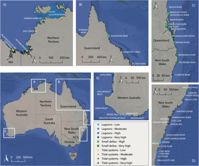
estimate areal water–air CH4 fluxes from 36 Australian estuaries and combine these with published CH4 emissions from an additional 11 Australian estuaries21,38 (total 47 estuaries, Fig. 1);

(2) evaluate the influence of estuary type and disturbance40 on CH4 concentrations and emissions from these 47 estuaries; and (3) use geomorphic and disturbance classifications for 971

Australian estuaries40 to scale CH4 emissions from these 47 estuaries to the whole of Australia to estimate Australia’s contribution to global estuarine CH4 emissions. We hypothesise that

both estuary type and the level of disturbance would significantly influence estuarine water CH4 concentrations and water–air CH4 fluxes, and that estuary type would interact with

disturbance to influence total CH4 emissions in Australia. We further hypothesise that CH4 fluxes per unit area from Australian estuaries would be lower than global estuary CH4 flux rates

because of the generally lower disturbance found in estuaries in Australia. By focusing on three geomorphic estuary types (lagoons, small deltas, and tidal systems) and four levels of

anthropogenic disturbance, the contribution of less disturbed estuaries to global CH4 emissions can be better estimated, lowering uncertainties in global estimates. RESULTS The results here

represent data for in-water CH4 concentrations and water–air CH4 fluxes measured in 36 sampled estuaries, combined with the same data published for 11 additional estuaries21,38 (details in

‘Methods’ section). The field campaign occurred over the 2017 to 2019 Australian summer seasons. The estuaries were grouped into three geomorphic types (lagoons, small deltas, and tidal

systems) and into four levels of anthropogenic disturbance (low, moderate, high, and very high)40. Together, the estuaries consist of 21 lagoons, 12 small deltas, and 14 tidal systems across

Australia (Table 1). INFLUENCE OF GEOMORPHOLOGY AND DISTURBANCE ON CH4 CH4 concentrations and water–air CH4 fluxes differed significantly (_p_ = 0.001) between the three estuary types (Fig.

 2a). Lagoons (_n_ = 751) had the highest mean (± standard error (SE)) CH4 concentration and water–air CH4 flux (95.8 ± 3.5 nmol l−1 and 183.9 ± 8 µmol CH4 m−2 d−1) driven by higher maximum

CH4 concentration and water–air CH4 flux (2196 nmol l−1 and 12,510 µmol CH4 m−2 d−1) compared to small deltas (_n_ = 719; max: 277 nmol l−1 and 680 µmol CH4 m−2 d−1) and tidal systems (_n_ =

 1138; max: 559 nmol l−1 and 1263 µmol CH4 m−2 d−1) (Fig. 2a and Table 2). Lagoons also had the highest median concentrations and fluxes, indicating that the high mean water–air flux was not

only due to the extremely high outliers (Table 2). Small deltas had the smallest range and the lowest maximum CH4 concentration and water–air CH4 flux (Fig. 2a and Table 2). Although small

deltas and tidal systems had similar mean CH4 concentrations, the mean water–air CH4 flux was 16% higher in tidal systems compared to small deltas (Fig. 2a and Table 2). Across all

estuaries, higher disturbance significantly increased (_p_ = 0.001) mean (± SE) CH4 concentration (Fig. 2b1) and water–air CH4 flux (Fig. 2b2) by approximately three times higher from the

moderate disturbance group (_n_ = 633; 28.2 ± 1.1 nmol l−1 and 66.4 ± 1.5 µmol CH4 m−2 d−1) to the very high disturbance group (_n_ = 888; 85.1 ± 1.7 nmol l−1 and 191.0 ± 3.0 µmol CH4 m−2 

d−1) (Table 2). However, low (_n_ = 356) and high (_n_ = 731) disturbance groups had similar CH4 concentrations and water–air CH4 fluxes (_p_ ≤ 0.202). CH4 concentrations and water–air CH4

fluxes in the low and high disturbance groups were significantly higher compared to the moderate disturbance group (_p_ ≤ 0.002) (Fig. 2b), which had the lowest CH4 concentration and

water–air flux (Table 2). Between estuary types, the effect of disturbance on CH4 concentration and water–air CH4 flux differed, but was generally stronger in the higher (high and very high)

disturbance groups (Fig. 3). CH4 concentration in the low disturbance lagoons (_n_ = 41) was significantly higher than in the moderate disturbance lagoons (_n_ = 161; _p_ = 0.053), but

significantly lower than in high (_n_ = 261) and very high disturbance lagoons (_n_ = 288; _p_ ≤ 0.017), for which CH4 concentrations were similar (_p_ = 0.712) (Fig. 3a1). The response of

water–air CH4 flux in lagoons to disturbance was slightly different from the response of CH4 concentration. Water–air CH4 fluxes in high and very high disturbance lagoons were significantly

higher than in low and moderate disturbance lagoons (_p_ ≤ 0.016), but water–air CH4 fluxes were similar between the low and moderate disturbance lagoons (_p_ = 0.298) (Fig. 3a2). The large

mean water–air CH4 flux in high-disturbance lagoons was driven by large outliers, as indicated by the lower median water–air flux for these systems (Fig. 3a2 and Table 2). In the moderate to

very high disturbance lagoons, outliers of CH4 concentrations and water–air CH4 fluxes were larger than those in small deltas and tidal systems, regardless of the disturbance group. These

large outliers in lagoons resulted in mean values that were higher than medians (Fig. 2a1, a2 and Table 2). In small deltas, CH4 concentration and water–air CH4 flux significantly increased

from the high (_n_ = 353) to very high disturbance systems (_n_ = 366; _p_ = 0.001) (Fig. 3b). In tidal systems, only very high disturbance systems (_n_ = 234) had significantly greater CH4

concentration and water–air CH4 flux compared to the other disturbance groups (_p_ = 0.001; moderate group _n_ = 472) (Fig. 3c). CH4 concentration and water–air CH4 flux in the low

disturbance tidal systems (_n_ = 315) were similar to those in high disturbance tidal systems (_n_ = 117; _p_ ≥ 0.444) (Fig. 3c and Table 2). It should be noted that the minimum salinity

measured in high-disturbance tidal system surveys was 21.640, which was associated with lower measured CH4 concentrations and water–air CH4 fluxes in these systems. EFFECT OF CLEARED

CATCHMENT LAND ON ESTUARY CH4 The mean percent of cleared catchment land increased with disturbance, from 10% in the low disturbance systems to 57% in very high disturbance systems (Table 

2), and for lagoons was correlated with a significant increase in CH4 concentrations (_n_ = 99; partial correlations; _r_ = 0.415 and _p_ = 0.001) (Fig. 4a) and water–air CH4 fluxes (_n_ = 

99; _r_ = 0.403 and _p_ = 0.001) (Fig. 4b). In tidal systems, CH4 concentrations also significantly increased with percent cleared catchment land (_n_ = 103; _r_ = 0.237 and _p_ = 0.017). In

contrast, increases in percent cleared catchment land in small deltas were associated with decreased CH4 concentrations (_n_ = 150; partial correlations; _r_ = −0.34 and _p_ = 0.001) and

water–air CH4 fluxes (_n_ = 150; _r_ = −0.22 and _p_ = 0.007), but no low or moderate disturbance systems were included, which limited the range of percent cleared catchments. SEASONAL

DIFFERENCES IN AUSTRALIAN ESTUARINE CH4 EMISSIONS To assess winter water–air CO2 fluxes, we calculated seasonal ratios using published summer and winter water–air CO2 fluxes from 13

estuaries (Supplementary Table 1) and averaged them according to each estuary type. We subsequently applied these ratios to the summer water–air CO2 fluxes observed in our current study to

estimate their winter water–air CO2 fluxes. Summer CH4 water–air fluxes in lagoons and small deltas were higher than in winter (means: lagoons: 0.21 vs. 0.12 mmol CH4 m−2 d−1 and small

deltas: 0.09 vs. 0.08 mmol CH4 m−2 d−1, Table 3), with mean seasonal ratios of 0.59 in the lagoons and 0.87 in the small deltas (Supplementary Table 2). In contrast, tidal system winter

water–air CH4 fluxes were higher than in summer (mean: 0.28 vs 0.09 mmol CH4 m−2 d−1, Table 3) with a mean seasonal ratio of 3.02 (Supplementary Table 2). Overall, Australian estuaries in

winter emit 0.16 ± 0.03 mmol CH4 m−2 d−1 (mean ± SE), 10.6% higher than in summer (Table 3). Using water–air flux rates measured over only the summer season, Australian estuaries emitted an

annual mean (± SE) of 18.17 ± 2.3 Gg CH4 yr−1 at a rate of 0.14 ± 0.03 mmol CH4 m−2 d−1 (Table 3), from a surface area of 39,390 km2 (Table 1). Tidal systems in summer contributed 69.8% of

annual emissions, followed by 29.3% by lagoons and 0.9% by small deltas (Table 3). The higher winter CH4 fluxes in tidal systems, combined with the large proportion of the total estuarine

surface area (89.9%), resulted in larger winter estuarine CH4 emissions in Australia (Table 3). The influence of tidal systems is reflected in annual CH4 emission from Australian estuaries

calculated using summer and winter CH4 fluxes, which was 68.1% higher than annual CH4 emission calculated using only summer CH4 fluxes. This is despite summer and winter averaged CH4 fluxes

being only 5.3% higher than the summer CH4 flux (Table 3). ANNUAL CH4 EMISSIONS FROM ALL AUSTRALIAN ESTUARIES We estimate mean (± SE) annual CH4 emissions (summer and winter) from Australian

estuaries to be 30.56 ± 12.43 (range: 24.53–36.7) Gg CH4 yr−1 (Table 3). Tidal systems accounted for the largest proportion of annual CH4 emissions (85%), followed by lagoons (13.9%) and

small deltas (1.1%). Interestingly, annual emissions of CH4 were 4.9% lower in tidal systems, 0.4% lower in small deltas, and 5.3% higher in lagoons than what would be expected based solely

on their surface area coverage (as indicated in Table 1). Annual CH4 emissions from lagoons generally increased with increasing disturbance, whereas emissions generally decreased with

increasing disturbance in tidal systems (Table 3). Mean (± SE) annual CH4 emissions in Australian estuaries were highest in the moderately disturbed estuaries (10.4 ± 2.18 Gg CH4 yr−1) and

lowest in the very high disturbance systems (3.99 ± 0.98 Gg CH4 yr−1). Of the total annual CH4 emissions in Australia, 73.8% were emitted by low and moderately disturbed tidal systems (Table

 3). DISCUSSION There was a strong geomorphic control on CH4 concentrations and water–air CH4 fluxes in Australian estuaries. All geomorphic estuary types were annual net sources of CH4 to

the atmosphere, but of the three estuary types, lagoons had the highest CH4 concentrations and water–air CH4 fluxes (Fig. 2a). The long residence times characteristic of lagoons41 due to low

river inflow37,42,43 and low tidal exchange40 likely enhanced the trapping of autochthonous and allochthonous organic matter4. This is consistent with lagoons having the highest dissolved

organic carbon (DOC) concentrations of all three estuary types40. Furthermore, the strongest inverse relationship between the water–air CH4 fluxes and tidal range was found in lagoons,

showing that water–air CH4 fluxes increased as the tidal range40 (Fig. 5b and Supplementary Notes) decreased (i.e. longer residence times). Lagoons also had the largest range in CH4

concentrations and water–air CH4 fluxes. This high variability in lagoons can be partly attributed to very high maximums for both CH4 concentration and water–air CH4 fluxes in the upstream

sections of the lagoons (Table 2). For example, although the mean per-estuary maximum CH4 flux in lagoons was ~3 times larger than in small deltas and tidal systems, the highest CH4 flux in

lagoons was ~18 times greater than in small deltas and ~10 times greater than in tidal systems (Table 2). This indicates that although mean flux rates in the lagoon basin section were

generally low, upstream lagoon riverine sections can have very high flux rates. The narrow upstream sections of lagoons have a higher density of terrestrial shoreline vegetation (visual

field and Google Earth observations), which would increase allochthonous carbon input44,45,46 and enhance CH4 emissions when the organic matter is decomposed4. CH4 emissions in upstream

sections of lagoons are likely to be further enhanced by low marine intrusion, as supported by the inverse trend between tidal range and water–air CH4 fluxes (Fig. 5b and Supplementary

Notes). Low marine intrusion would limit the availability of marine-derived sulphate, and reduce the competition between methanogens and sulphate-reducing bacteria, resulting in increased

methanogenesis4,47. Overall CH4 concentrations and water–air CH4 fluxes in small deltas and tidal systems were lower than in lagoons likely due to shorter water residence times41, resulting

in less time for organic matter degradation. Decreasing DOC concentrations alongside increasing dissolved inorganic carbon (DIC) concentrations from lagoons to small deltas and tidal

systems40 likely reflected laterally imported DIC and CH4 from shoreline habitats to estuarine waters via tidal pumping32,48. Shoreline habitats trap DOC and release DIC into the water

column. Increased lateral export of CH4 (and DIC) was likely related to the strong hydrological connectivity of tidal systems and deltas with adjacent mangroves and saltmarshes49,50. High

lateral inputs are consistent with the positive relationship between tidal range40 and CH4 concentration and water–air CH4 fluxes (Fig. 5c and Supplementary Notes) in the small deltas

studied here, and in other small deltas51 and tidal systems52,53. Mean CH4 concentrations were similar between the small deltas and tidal systems, but mean water–air CH4 fluxes in tidal

systems were higher compared to small deltas (Fig. 2a). Higher water–air CH4 fluxes in tidal systems are linked to higher gas transfer velocities40 driven by faster water current velocities

compared to other estuary types40. CH4 concentrations and water–air CH4 fluxes generally increased from the moderate, to high, to very high disturbance groups (Fig. 2b). Enhanced CH4

concentrations and water–air CH4 fluxes have been found in impacted estuaries with higher pollution inputs (e.g. wastewater)39,54 and higher DOC concentrations39,55. Within estuary-type

classes, CH4 concentrations and water–air CH4 fluxes generally increased in higher disturbance systems (Fig. 3). However, the direction of the relationship between DOC concentration and

disturbance was estuary-type specific40. Estuary type also influenced the direction of relationships between percent cleared catchment land and CH4 concentration and to water–air CH4 flux

(i.e. estuary type modified the effect of disturbance on CH4 concentrations and water–air CH4 fluxes). High and very high disturbance lagoons generally had higher CH4 concentrations and

water–air fluxes than low and moderate disturbance lagoons (Fig. 3a); CH4 concentrations and water–air CH4 fluxes increased with percent cleared catchment land (Fig. 4). DOC concentrations40

were significantly correlated to CH4 concentrations (_r_ = 0.29 and _p_ = 0.004) and water–air CH4 fluxes (_r_ = 0.23 and _p_ = 0.021) in lagoons. Similar partial correlation was found for

DOC concentrations and CH4 concentrations (_r_ = 0.21 and _p_ = 0.036) or water–air CH4 fluxes (_r_ = 0.2 and _p_ = 0.043) in tidal systems. However, high and very highly disturbed lagoons

had generally lower DOC40 than the low and moderate disturbance lagoons. These trends suggest that DOC concentrations did not drive increased CH4 in higher disturbance lagoons. Rather,

catchment land use changes, and associated variations in riverine input, likely affected organic matter quality and biogeochemical processes, including methanogenesis56,57,58. Long residence

times in lagoons2 have been shown to simultaneously enhance allochthonous organic matter degradation and autochthonous organic matter production56, thereby enhancing CH4 production. Changes

in CH4 concentrations and water–air CH4 fluxes with increasing disturbance in the tidal systems were less obvious and were only significantly higher in the very high disturbance systems

compared to the lower disturbance systems (Fig. 3c). The less pronounced disturbance effect on CH4 in tidal systems may reflect the larger tidal range40 and associated larger water exchange

compared to other estuary types, which in turn may mask any disturbance effect. However, low to highly disturbed tidal systems were all located in the largely undeveloped areas along the

northern coastline36, where catchment vegetative cover is high36. Therefore, low CH4 concentrations and water–air CH4 fluxes in the low to high-disturbance tidal systems could be due to

naturally low allochthonous inputs from the catchments. In contrast, the very high disturbance tidal systems were located in heavily developed areas (i.e. Moreton Bay (Queensland), Port

Philip Bay (Victoria), and Botany Bay (New South Wales)). Australian estuaries overall emitted more CH4 in winter than in summer. This was driven by relatively high winter CH4 flux rates in

tidal systems which account for 89.9% of Australian estuarine surface area. Lagoons and small deltas emitted less CH4 in winter than in summer, but account for only 10.1% of estuarine

surface area in Australia (Table 1). The impact of lagoons and small deltas on annual CH4 emissions was therefore relatively low (Table 3). Seasonal differences in CH4 emissions have not

been extensively studied but a comparison of the Australian estuaries with estuaries in other countries suggests that seasonal trends differ between systems. For example, water–air CH4

fluxes in the Rhine estuary in Germany were higher in the summer (median: 600 nmol l−1) than in the winter (median: 310 nmol l−1)7. Similarly, summer water–air CH4 fluxes were two times

higher than winter fluxes in the tidal Tay estuary in the UK (summer: 0.35 g C m−2 yr−1, winter: 0.15 g C m−2 yr−1)59, and there were no seasonal differences in three other European tidal

systems (Guadalquivir60, Scheldt, and Gironde)7. Seasonal temperature differences have been proposed to influence CH4, with higher microbial activity in warmer, summer months enhancing

fluxes61. However, this is inconsistent with the observations in the current study, where overall fluxes were higher in winter. This may reflect less seasonal variation in temperatures in

the tidal systems which are mostly in the tropics. Geomorphic factors (e.g. tidal influence) may have also influenced the seasonal differences in CH4 emissions in tidal systems (and the

other estuary types) such as changes in rainfall, lateral inputs, and biological activity, not just temperature. Shallower lagoons and small deltas may also be more sensitive to temperature

changes due to a smaller buffering capacity compared to the larger tidal systems (Supplementary Notes). To account for seasonal water–air CH4 flux variability62, we applied the minimum and

maximum seasonal ratios (Supplementary Table 2) to the summer flux rates to obtain a range of winter flux rates, which were used to calculate lower and higher estimates of annual CH4

emissions (Table 3). While we observed seasonal variability in Australian estuaries, the spatial variability within individual estuaries (overall mean of the minimum to mean of the maximum

flux rate: 32.9–628.3 µmol CH4 m−2 d−1, difference of 595.4 µmol CH4 m−2 d−1) was substantially greater than seasonal variability (difference between the mean of summer and mean of winter

estuary mean flux rates: 15.2 µmol CH4 m−2 d−1), indicating that spatial variability along salinity gradients is more important than temporal variability (i.e. summer and winter differences)

in determining CH4 emissions from Australian estuaries. The effect of salinity on CH4 was supported by significantly decreased CH4 concentration and water–air CH4 flux with increasing

salinity in all estuary types (Supplementary Notes and Supplementary Fig. 4). Episodic events may be an important source of variability63,64, but were not captured in this study. Within each

estuary-type class, the difference between the mean minimum rates of each estuary and mean maximum rates of each estuary in water–air CH4 fluxes was 15-fold in lagoons (66.9 to 995 µmol CH4

 m−2 d−1), 95-fold in small deltas (3.8–362 µmol CH4 m−2 d−1), and 46-fold in tidal systems (6.7–308 µmol CH4 m−2 d−1) (Table 2). Although the difference in minimum and maximum flux rates

between lagoons had the smallest magnitude of increase compared to the other two estuary types (15-fold compared to 95-fold and 46-fold), they had the highest minimum and maximum flux rates,

and the largest range of flux rates (Table 2). This shows that the relationship between CH4 flux rates and salinity depended on the estuary type and had a greater impact on overall estuary

CH4 emissions than seasonal variability. Therefore to capture the variations in CH4 concentrations in estuaries, we used arithmetic means instead of medians. This approach allowed CH4

concentrations and flux rates to be compared more effectively, incorporating the higher concentrations and flux rates in upper estuarine regions that would otherwise have been missed. There

are two recent compilations of global estuarine CH4 emissions3,8 which can be compared to the Australian estuarine CH4 emissions estimated in the current study. Firstly, our mean (± SE)

Australian estuarine emission was compared to the mean (± confidence interval) from Rosentreter et al.3. Because Rosentreter et al.8 report median using a bootstrapping approach, their mean

global estuary emissions were recalculated for tidal systems and deltas (mean 0.26 Tg CH4 yr−1 using 0.15 mmol CH4 m−2 d−1 and a global surface area of 294,956 km2) and lagoons (mean 0.17 Tg

CH4 yr−1 using 0.16 mmol CH4 m−2 d−1 and a global surface area of 179,946 km2) for the purpose of better comparison with means in this study (Fig. 6a). Mean water–air CH4 fluxes in

Australian low and moderately disturbed lagoons, high and very high disturbed small deltas, and low, moderately, and high disturbance tidal systems (Table 3) were lower than mean global

estimates (all estuary types, 0.15 ± 0.02 mmol CH4 m−2 d−1) from ref. 3, and also lower than global mean fluxes in lagoons (0.16 ± 0.06 mmol CH4 m−2 d−1) and global mean fluxes in tidal

systems and deltas (0.15 ± 0.03 mg CH4 m−2 d−1) from ref. 8. (Fig. 6a). This is significant because these Australian estuary disturbance classes account for 89.8% of the total estuarine

surface area in Australia (Table 1 and Fig. 6b). Only the high (0.24 mmol CH4 m−2 d−1) and very high (0.24 mmol CH4 m−2 d−1) disturbed lagoons and very high tidal systems (0.44 mmol CH4 m−2 

d−1, Table 3) had water–air fluxes greater than global water–air fluxes3,8. However, these systems make up only 8.6% of total estuarine surface area in Australia, and make only a small

contribution (17.8%) to total estuary emissions in Australia (Fig. 6b). In addition, many of the global studies used an open water parameterisation (i.e. ref. 65). Had we only used the

Wanninkhof65 parameterisation, instead of an average of five parameterisations, our Australian estuarine CH4 fluxes would have been even lower. Lower water–air CH4 fluxes in the majority of

Australia estuaries compared to global fluxes probably reflect an overall lower catchment disturbance in Australia, which was captured in our sampling design and upscaling. Lower catchment

disturbance is associated with low population density (3.3 people km−2)35 and the delivery of lower riverine loads of carbon and nutrients64,66 into Australian estuaries. In fact, Australia

is part of ~34% of global coastal regions that are classified as less than moderately disturbed (>40% intact)34. Most of Australia’s annual estuarine CH4 emissions come from low and

moderately disturbed tidal systems (73.8%, 22.55 Gg CH4 yr−1, Table 3) which are mostly found in remote northern Australia. This highlights the need to not only include a broad range of

geomorphic types, but also for disturbance when upscaling estuarine CH4 emissions. Australia’s estuaries have lower water–air CH4 fluxes than estuaries globally due to lower disturbance, and

total emissions are driven by low and moderately disturbed tidal systems in remote northern Australia. Assuming Australia is a good analogue for the ~34% of global coastal regions

classified as less than moderately disturbed (>40% intact)34, and given that recent global estuarine CH4 emission estimates3,8 do not include disturbance in their upscaling, global

estuarine CH4 emissions are probably over-estimated. This highlights the need to include a broader range of geomorphic types and disturbance levels when measuring water–air CH4 fluxes and

upscaling regional and global estuarine CH4 emissions. METHODS FIELDWORK DESCRIPTION 36 estuaries were sampled for in-water CH4 concentrations, physical parameters (water current velocity,

water depth, and wind speed), and physicochemistry (salinity, temperature, pH, and dissolved oxygen) in the austral spring-summer season (2017–2019). The same data for 11 estuaries sampled

under similar seasonal conditions were sourced from refs. 38,21, where the required parameters were available. The spatial surveys encompassed 21 estuaries along the New South Wales

coastline (Merimbula to Brunswick Heads, Nov to Dec 2017), one in southeast Queensland (Moreton Bay, Oct 2018), seven along the north coast of Australia (Karumba, Queensland to Wyndham,

Western Australia, Oct to Dec 2018), and seven in southwest Western Australia (Perth to Albany, Feb to Mar 2019) (Fig. 1 and Supplementary Table 3). Data for an additional eight estuaries in

southeast Queensland were derived from ref. 21 (Sept to Oct 2014) and three in Queensland from ref. 38 (Oct 2016) (Fig. 1 and Supplementary Table 3). ESTUARY CLASSIFICATION SCHEMES

Estuaries were selected to cover a large range of disturbance and geomorphic types according to the classifications of NLWRA36 and ref. 2, respectively. NLWRA36 assessed 971 Australian

estuaries and described four disturbance classes (low (near-pristine), moderate (relatively unmodified), high (modified), and very high (extensively modified)), based on changes in catchment

land use, estuary use, and ecology. The global estuarine typology of ref. 2 details three geomorphic types found in Australia: 1) lagoons (including Intermittently Closed or Open Lakes and

Lagoons (ICOLLs) and estuaries with a central basin morphology), 2) small deltas, and 3) tidal systems (including drowned river valleys and tidal embayments) based on tidal influence,

sedimentation, and hydrology. However, the existing classification of Australian estuaries2 did not match our observations of satellite imagery, because it was developed with a low spatial

resolution (0.5°, or 50 km). Therefore, we used the updated classification database by ref. 40, which categorised estuaries using the classification by ref. 2 combined with the estuarine

disturbance database of NLWRA36. The distribution of estuary types across Australia corresponds to the tidal ranges along their respective coastlines (Supplementary Fig. 3). In northern

Australia, macro-tidal regions are dominated by tidal systems while in the micro-tidal regions of southern Australia, lagoons are more prevalent. Our estuary selection includes all three

estuary types with all four disturbance groups, except for low and moderate disturbance in small deltas (Table 1). The estuaries sampled and included in this study represent 12.5% of the

total Australian estuarine surface area, consisting of 19.8% of lagoons, 10.3% of small deltas, and 11.8% of tidal systems in Australia (Table 1). UNDERWAY DATA MEASUREMENTS Boat-based

survey transects were carried out in each estuary starting after high tide, from the marine mouth (~35 salinity) to the riverine-freshwater endmember (~2 salinity). Despite the aim of

sampling a minimum salinity of 2, some estuary surveys were ended at higher salinities than 2 due to shallow depths and obstacles impeding further progress. The surveys were conducted in

daylight hours, typically over a single day, with the larger estuaries requiring multiple days but no more than five days. A cruising speed of ~8 km h−1 was maintained whenever possible to

ensure spatial and temporal consistency while the survey was underway. As a result, measurements taken in the estuary surveys reflect the spatial variation of parameters along the estuarine

gradient (from marine to riverine). Underway physicochemical data and _p_CH4 were measured via an integrated water-gas loop along the survey transect (Supplementary Fig. 1). Sample water was

pumped from a depth of 0.5 m to 1 m using a 12 V pump with back-flow prevention (800GPH, Rule) and screen-filtered (High-flow filter basket, Ozito); before splitting into: (1) a flowthrough

receptacle housing a physicochemical sonde (HL4, Hydrolab) recording per-minute measurements of temperature (±0.1 °C), salinity (±0.5%), pHNBS (±0.2), and percent saturation dissolved

oxygen (DO%sat, ±2%), and (2) a pair of interconnected showerhead exchangers (RAD Aqua, Durridge) where dissolved gases in the incoming sample water were equilibrated with the exchanger

headspace, and the dried air (Drierite) analysed in-line with a Picarro G−2508 cavity ring-down spectrometer (CRDS) measuring in-air CH4 (ppmv)67. Corrections for water vapour pressure were

applied to CH4 dry mole fractions using methods of ref. 68, after which CH4 dry mole fractions were converted into in-water CH4 partial pressure (µatm) and concentration (nmol l−1). The

physicochemical sonde was calibrated regularly in the field, and the CRDS was serviced and calibrated by the manufacturer (±0.3 ppb) (Picarro, USA). Physicochemical data is presented in ref.

40. COLLECTION OF DISCRETE WATER SAMPLES, MORPHOLOGICAL, AND METEOROLOGICAL DATA Measurements for physical (water depth and current velocity) and meteorological data (barometric pressure,

air temperature, and true wind speed) were collected concurrently with underway measurements (CH4 concentrations and physicochemistry) at the start and end of surveys and at salinity

intervals of 5. When salinity change was smaller than 5 per hour, samples were taken every hour instead (i.e. every 8 km travelled along the estuary) to account for changes in other

estuarine parameters. Water samples for CH4 were processed immediately after collection. At each water sampling site, barometric pressure (±0.5 hPa @20 °C), true wind speed (±5% @10 m s−1),

and air temperature (±0.1 °C @20 °C) were measured using a vessel-mounted weather station (200WX, Airmar) 3 m above the water surface. Water depth was measured using a hull-mounted acoustic

transducer (Airmar), and water current velocity was measured using a sub-surface drifter and the differential GPS-assisted Lagrangian method (adapted from Wetzel and Likens69). Current

velocity measurements represented flow rates of the ebbing tide. In the smaller NSW lagoons, in-situ meteorological and water depth measurements were not collected. Instead, averaged daily

meteorological measurements were obtained from the closest Bureau of Meteorology weather station70 and averaged water depth data was taken from ref. 71. Physical and meteorological data are

presented in ref. 40. Water samples for CH4 concentration were taken in the nine smaller, closed lagoons where the CRDS-equipped vessel could not be used for underway CH4 measurements. Water

samples for CH4 analysis (6 ml) were syringe-filtered (0.22 µm PTFE Minisarts, Sartorius) at each sampling interval into duplicate 12 ml exetainers (Labco) pre-purged with N2 with a needle

through the septa72, inverted, and refrigerated (4 °C) until analysis. The exetainers were loaded with 20 µl saturated HgCl2 solution and pre-weighed before sample collection. The exetainers

with samples were weighed again before analysis to determine the sample volume21. CH4 concentrations in the headspace (coefficient of variation: ±5.2%) at room temperature were subsequently

measured by gas chromatography (Shimadzu GC-9A) with a flame ionisation detector21. Measured gas-phase concentrations were converted into liquid-phase concentrations using the solubility

calculations of ref. 73. CH4 concentrations were linearly interpolated between sampling points into per-minute measurements along the survey transect to maintain spatial and temporal

consistency between estuaries. Using interpolated CH4 data, instead of averaged data, more accurately represented spatial gradients across lagoon basins. The percentage of the estuary

catchment cleared of natural vegetation (percent cleared catchment land) was based on existing data for New South Wales estuaries71, southeast Queensland estuaries74, Broke Inlet (Department

of Water and Environmental Regulation (DWER), _unpublished data_), Irwin Inlet75, Walpole Inlet76, Hardy Inlet77, Wilson Inlet (DWER, _unpublished data_), Swan River78, Leschenault Inlet79,

Johnstone River80, Constant Creek81, Fitzroy River82, Ord River estuaries83, and for the other north Australian estuaries36 (Supplementary Table 4). Mean tidal range data for the study

estuaries were obtained from NLWRA36. WATER–AIR CH4 FLUX CALCULATIONS The per-minute water–air CH4 flux (_F_CH4; µmol CH4 m−2 d−1) was calculated using equation 1:

$${F{{\rm{CH}}}}_{4}=k{{{\rm{K}}}}_{0}\left({C}_{{water}}-{C}_{{air}}\right)$$ where _k_ is the gas transfer velocity of CH4 (m d−1) and _K_0 is the CH4 solubility coefficient (mol l−1 

atm−1)73 expressed as functions of temperature and salinity, and _C_water and _C_air are the partial pressure of CH4 (µatm) in water and air, respectively65. Atmospheric CH4 was taken to be

the mean annual concentration of 1.86 ppm in 201884. _k_600 was calculated based on five parameterisations obtained from the literature25,26,27,65,85:

$${k}_{600}=-0.08+0.26v+0.83{u}_{10}+0.59h$$ (2) Rosentreter et al.27 $${k}_{600}=1+1.719{v}^{0.5}{h}^{-0.5}+2.58{u}_{10}$$ (3) Borges et al.25

$${k}_{600}=0.314{{u}_{10}}^{2}-0.436{u}_{10}+3.99$$ (4) Jiang et al.85 $${k}_{600}=0.77{v}^{0.5}{h}^{-0.5}+0.266{u}_{10}$$ (5) Ho et al.26

$$k=0.251{{u}_{10}}^{2}{\left(\frac{{Sc}}{660}\right)}^{-0.5}$$ (6) Wanninkhof65. In the first four parameterisations (Eqs. 2–5), _k_600 represents the gas transfer velocity normalised to

Schmidt number of 600, _v_ is water current velocity (cm h−1), _U_10 is windspeed at a 10 m height (m s-1)86, and _h_ is water depth (m). The parameterisation by Wanninkhof65 (Eq. 6)

calculated for _k_ to the Schmidt number at the measured temperature and salinity, which was then normalised to _k_600 using equation 765:

$${k}_{600}=k{\left(\frac{600}{{Sc}}\right)}^{-0.5}$$ where _Sc_ was the Schmidt number and assuming a Schmidt exponent of −0.5 due to generally high water turbulences by tidal currents87

found in estuaries. Because _k_ was used to calculate the water–air flux of CH4, _k_600 calculated using the other 4 parameterisations (Eqs. 2–5) were converted into _k_ by rearranging

equation 7. These parameterisations were chosen to reflect mangrove-dominated26,27, tidal25, lagoonal85, and marine-dominated65 environments found in estuaries. Although the parameterisation

by Wanninkhof65 was designed for marine open-water environments, we argue that it would be representative of the large, open tidal estuaries found in many tidal systems around Australia.

Many estuary studies included in global estimates also include this parameterisation, making this current study comparable to other published estimates. Water–air CH4 fluxes in the eight

southeast Queensland estuaries21 were recalculated using the five parameterisations to ensure consistency. Recalculation was not possible for the three north Queensland estuaries38 because

water depth and current velocity data were unavailable. However, there was only one of these three estuaries in any given disturbance group and/or estuary type (i.e. moderate and high

disturbance tidal system, and a high disturbance small delta, Table 1) and therefore, they should not introduce any systemic bias. DATA PROCESSING AND STATISTICS Per-minute CH4 concentration

and water–air CH4 flux calculations were reduced to 5-min averages to simplify data processing and analysis while maintaining high resolution and data features along the survey transects.

Kolmogorov-Smirnov test for normality and Levene’s tests for homoscedasticity returned significant results and together with an unbalanced study design, justified a non-parametric analysis

approach. CH4 concentrations and water–air CH4 fluxes were not power-transformed but were normalised (_z_-score) before analysis. Not transforming the dataset retains the original

heterogeneity of the mean-variance relationship and the spatial scale along the estuarine gradient, and avoids an inflated type I error as a result88. Differences in CH4 concentrations and

water–air CH4 fluxes between estuary types (3 factors) and disturbance groups (4 factors) were analysed for significance (_α_ = 0.05; two-tailed) using the PERMANOVA procedure (Primer v7

with PERMANOVA+, PRIMER-e). Salinity was included as a covariate in the PERMANOVA analyses to account for possible effects on CH4. The effect of salinity was confirmed by significant

correlations between CH4 and salinity (Pearson’s correlation analysis, _α_ = 0.05, SPSS v25, IBM). Because PERMANOVA draws significance from tests based on permutations between datapoints,

significant differences can be identified where descriptive statistics appear similar. 9999 permutations were executed using type I sum of squares with residuals under a reduced model.

Significant differences between estuary types and the effect of disturbance within each estuary type were further investigated using pairwise tests (Primer v7 with PERMANOVA+, PRIMER-e).

Correlations of CH4 concentrations and water–air CH4 fluxes with physicochemistry (temperature, pH, dissolved oxygen, and salinity40), percent cleared catchment land, tidal range, and DOC

concentration40 were power-transformed, normalised (_z_-score), and analysed using partial correlation (_α_ = 0.05) while controlling for salinity as a covariate (SPSS v25, IBM). Given that

finding the drivers of CH4 concentration and CH4 emissions was the focus of this study, partial correlation analysis was chosen over exploratory multivariate methods such as Principal

Component Analysis (PCA), allowing for targeted testing for correlations between variables and CH4. UPSCALING ESTUARINE CH4 EMISSIONS TO THE AUSTRALIAN CONTINENT Published summer and winter

water–air CH4 flux rates were available for ten21,38 Australian small deltas and tidal systems. These seasonal CH4 flux rates were used to calculate the seasonal ratios (winter:summer) for

small deltas and tidal systems (Supplementary Table 1). The relationship between small delta CO240 and CH4 seasonal ratios (_S_CH4 = 0.6106(_S_CO2) + 0.2062, Supplementary Fig. 2) was

applied to estimate seasonal CH4 ratios for lagoons (Supplementary Table 2). Indeed, the relationship between CO2 and CH4 for small deltas may not apply to lagoons in the same way.

Therefore, the calculated seasonal ratios for lagoons should be interpreted with caution. After which, mean _S_CH4 were calculated for each estuary type and applied to summer water–air CH4

fluxes to obtain winter flux rates of the 47 study estuaries (Table 3). The sensitivity of winter flux rates on annual CH4 emission in Australian estuaries was also tested by applying the

range of _S_CH4 to the annual CH4 emission upscaling exercise (Table 3)62. The sensitivity range is reported alongside the overall annual CH4 emission estimate. Mean and median annual CH4

emissions and their uncertainties (standard error) from all Australian estuaries (_n_ = 971; Supplementary Fig. 3) were calculated by scaling disturbance-specific mean water–air CH4 fluxes

(µmol CH4 m−2 d−1) averaged per-estuary into the mean estuary type flux rate from the 47 study estuaries, and applied across the relevant total Australian estuarine surface areas (Table 1)

of these geomorphic and disturbance types (area-weighting). Small deltas with low to moderate disturbance were not available for this study. The exclusion of these estuary types would result

in an overestimation of CH4 emissions from small deltas, but the impact is likely to be negligible, given that low and moderate disturbance small deltas account for only 0.5% of Australian

estuarine surface area (all small deltas account for 1.5%). The mean and median small delta CH4 flux were used in their place when upscaling annual CH4 emissions. REPORTING SUMMARY Further

information on research design is available in the Nature Portfolio Reporting Summary linked to this article. DATA AVAILABILITY The methane data measured and used in this study can be found

in the data repository FigShare under the accession code https://doi.org/10.6084/m9.figshare.25933060. Source data for figures can be found in Supplementary Data 1. REFERENCES * Forster, P.

et al. The Earth’s energy budget, climate feedbacks, and climate sensitivity. In Climate Change 2021: The Physical Science Basis. Contribution of Working Group I to the Sixth Assessment

Report of the Intergovernmental Panel on Climate Change. Cambridge University Press, Cambridge, United Kingdom and New York, NY, USA (2021). * Dürr, H. H. et al. Worldwide typology of

nearshore coastal systems: defining the estuarine filter of river inputs to the oceans. _Estuar. Coasts_ 34, 441–458 (2011). Article  Google Scholar  * Rosentreter, J. A. et al. Half of

global methane emissions come from highly variable aquatic ecosystem sources. _Nat. Geosci._ 14, 225–230 (2021). Article  CAS  Google Scholar  * Borges, A. V. & Abril, G. Carbon dioxide

and methane dynamics in estuaries. In _Treatise on Estuarine and Coastal Science_ (eds. Wolanski, E. & McLusky, D.) vol. 5 119–161 (Waltham: Academic Press, 2011). * Bange, H. W.,

Bartell, U. H., Rapsomanikis, S. & Andreae, M. O. Methane in the Baltic and North Seas and a reassessment of the marine emissions of methane. _Glob. Biogeochem. Cycles_ 8, 465–480

(1994). Article  CAS  Google Scholar  * Upstill-Goddard, R. C., Bames, J., Frost, T., Punshon, S. & Owens, N. J. P. Methane in the southern North Sea: low-salinity inputs, estuarine

removal, and atmospheric flux. _Glob. Biogeochem. Cycles_ 14, 1205–1217 (2000). Article  CAS  Google Scholar  * Middelburg, J. J. et al. Methane distribution in European tidal estuaries.

_Biogeochemistry_ 59, 95–119 (2002). Article  Google Scholar  * Rosentreter, J. A. et al. Coastal vegetation and estuaries collectively are a greenhouse gas sink. _Nat. Clim. Chang_. (2023).

* Woodwell, G. M., Rich, P. H. & Hall, C. A. Carbon in estuaries. _Brookhaven Symposium on Biology_ 30, (1973). * Laruelle, G. G., Rosentreter, J. A. & Regnier, P.

Extrapolation-based regionalized re-evaluation of the global estuarine surface area. _Estuar. Coasts_ 1–33 (2023). * Abril, G. & Borges, A. V. Carbon dioxide and methane emissions from

estuaries. In _Greenhouse Gas Emissions—Fluxes and Processes_ (eds. Tremblay, A., Varfalvy, L., Roehm, C. & Garneau, M.) 187–207 (Springer, 2005). * Reeburgh, W. S. Oceanic methane

biogeochemistry. _ChemInform_ 38, 486–513 (2007). Article  Google Scholar  * Kelley, C. A., Martens, C. S. & Chanton, J. P. Variations in sedimentary carbon remineralization rates in the

White Oak River estuary, North Carolina. _Limnol. Oceanogr._ 35, 372–383 (1990). Article  CAS  Google Scholar  * Borja, A. et al. Classifying ecological quality and integrity of estuaries.

in _Treatise on Estuarine and Coastal Science_ (eds. Wolanski, E. & McLusky, D.) Vol. 1, 125–162 (Waltham: Academic Press, 2012). * Harris, G. P. Biogeochemistry of nitrogen and

phosphorus in Australian catchments, rivers and estuaries: Effects of land use and flow regulation and comparisons with global patterns. _Mar. Freshw. Res._ 52, 139–149 (2001). Article  CAS

  Google Scholar  * Painting, S. J. et al. Assessing the impact of nutrient enrichment in estuaries: Susceptibility to eutrophication. _Mar. Pollut. Bull._ 55, 74–90 (2007). Article  CAS 

Google Scholar  * Cloern, J. E. Our evolving conceptual model of the coastal eutrophication problem. _Mar Ecol Prog Ser_ 210, 223–253 (2001). Article  CAS  Google Scholar  * Burgos, M.,

Sierra, A., Ortega, T. & Forja, J. M. Anthropogenic effects on greenhouse gas (CH4 and N2O) emissions in the Guadalete River Estuary (SW Spain). _Sci. Total Environ._ 503–504, 179–189

(2015). Article  Google Scholar  * Cotovicz, L. C. et al. Spatio-temporal variability of methane (CH4) concentrations and diffusive fluxes from a tropical coastal embayment surrounded by a

large urban area (Guanabara Bay, Rio de Janeiro, Brazil). _Limnol. Oceanogr._ 61, S238–S252 (2016). Article  Google Scholar  * DelSontro, T., del Giorgio, P. A. & Prairie, Y. T. No

longer a paradox: the interaction between physical transport and biological processes explains the spatial distribution of surface water methane within and across lakes. _Ecosystems_ 21,

1073–1087 (2018). Article  CAS  Google Scholar  * Wells, N. S. et al. Changing sediment and surface water processes increase CH4 emissions from human-impacted estuaries. _Geochim. Cosmochim.

Acta_ 280, 130–147 (2020). Article  CAS  Google Scholar  * Al-Haj, A. N. & Fulweiler, R. W. A synthesis of methane emissions from shallow vegetated coastal ecosystems. _Glob. Chang.

Biol._ 26, 2988–3005 (2020). Article  Google Scholar  * Harris, P. T. & Heap, A. D. Environmental management of clastic coastal depositional environments: Inferences from an Australian

geomorphic database. _Ocean Coast. Manag._ 46, 457–478 (2003). Article  Google Scholar  * Harris, P. T. et al. Classification of Australian clastic coastal depositional environments based

upon a quantitative analysis of wave, tidal, and river power. _J. Sediment. Res._ 72, 858–870 (2002). Article  Google Scholar  * Borges, A. V. et al. Variability of the gas transfer velocity

of CO2 in a macrotidal estuary (the Scheldt). _Estuaries_ 27, 593–603 (2004). Article  CAS  Google Scholar  * Ho, D. T. et al. Influence of current velocity and wind speed on air-water gas

exchange in a mangrove estuary. _Geophys. Res. Lett._ 43, 3813–3821 (2016). Article  Google Scholar  * Rosentreter, J. A. et al. Spatial and temporal variability of CO2 and CH4 gas transfer

velocities and quantification of the CH4 microbubble flux in mangrove dominated estuaries. _Limnol. Oceanogr._ 62, 561–578 (2017). Article  Google Scholar  * Rosentreter, J. A., Wells, N.

S., Ulseth, A. J. & Eyre, B. D. Divergent gas transfer velocities of CO2, CH4, and N2O over spatial and temporal gradients in a subtropical estuary. _J. Geophys. Res. Biogeosci._ 126,

1–21 (2021). Article  Google Scholar  * Borges, A. V. et al. Effects of agricultural land use on fluvial carbon dioxide, methane and nitrous oxide concentrations in a large European river,

the Meuse (Belgium). _Sci. Total Environ._ 610–611, 342–355 (2018). Article  Google Scholar  * Maeck, A. et al. Sediment trapping by dams creates methane emission hot spots. _Environ. Sci.

Technol._ 47, 8130–8137 (2013). Article  CAS  Google Scholar  * Koné, Y. J. M., Delille, Á. B., Borges, A. V. & Abril, G. Seasonal variability of methane in the rivers and lagoons of

Ivory Coast (West Africa). _Biogeochemistry_ 100, 21–37 (2010). Article  Google Scholar  * Call, M. et al. Spatial and temporal variability of carbon dioxide and methane fluxes over

semi-diurnal and spring-neap-spring timescales in a mangrove creek. _Geochim. Cosmochim. Acta_ 150, 211–225 (2015). Article  CAS  Google Scholar  * Call, M. et al. High pore-water derived

CO2 and CH4 emissions from a macro-tidal mangrove creek in the Amazon region. _Geochim. Cosmochim. Acta_ 247, 106–120 (2019). Article  CAS  Google Scholar  * Williams, B. A. et al. Global

rarity of intact coastal regions. _Conserv. Biol._ 36, 1–12 (2022). Article  Google Scholar  * Regional population, Australia, 2020−2021. Australian Bureau of Statistics

https://www.abs.gov.au/statistics/people/population/regional-population/2020-21 (2022). * NLWRA. Australian Catchment, River and Estuary Assessment 2002. Vol. 1 (National Land and Water

Resources Audit, Commonwealth Government, 2002). * McSweeney, S. L., Kennedy, D. M., Rutherfurd, I. D. & Stout, J. C. Intermittently closed/open lakes and lagoons: their global

distribution and boundary conditions. _Geomorphology_ 292, 142–152 (2017). Article  Google Scholar  * Rosentreter, J. A., Maher, D. T., Erler, D. V., Murray, R. H. & Eyre, B. D. Factors

controlling seasonal CO2 and CH4 emissions in three tropical mangrove-dominated estuaries in Australia. _Estuar. Coast. Shelf Sci._ 215, 69–82 (2018). Article  CAS  Google Scholar  * Looman,

A. et al. Dissolved carbon, greenhouse gases, and δ13C dynamics in four estuaries across a land-use gradient. _Aquat. Sci._ 81, 1–15 (2019). Article  Google Scholar  * Yeo, J. Z.-Q.,

Rosentreter, J. A., Schulz, K. G., Eyre, B. D. & Oakes, J. M. High carbon dioxide emissions from Australian estuaries driven by geomorphology and climate. _Nat. Commun_. 15, (2024). *

Laruelle, G. G. et al. Global multi-scale segmentation of continental and coastal waters from the watersheds to the continental margins. _Hydrol. Earth Syst. Sci._ 17, 2029–2051 (2013).

Article  Google Scholar  * Kennish, M. J. & Paerl, H. W. _Coastal lagoons: critical habitats of environmental change_. _Coastal Lagoons: Critical Habitats of Environmental Change_

(2010). * de Brito, A. N., Fragoso, C. R. & Larson, M. Tidal exchange in a choked coastal lagoon: a study of Mundaú Lagoon in northeastern Brazil. _Reg. Stud. Mar. Sci._ 17, 133–142

(2018). Google Scholar  * Brett, M. T. et al. How important are terrestrial organic carbon inputs for secondary production in freshwater ecosystems? _Freshw. Biol._ 62, 833–853 (2017).

Article  CAS  Google Scholar  * Krauss, K. W. et al. The role of the upper tidal estuary in wetland blue carbon storage and flux. _Glob. Biogeochem. Cycles_ 32, 817–839 (2018). Article  CAS

  Google Scholar  * Meyer, J. L., Wallace, J. B. & Eggert, S. L. Leaf litter as a source of dissolved organic carbon in streams. _Ecosystems_ 1, 240–249 (1998). Article  CAS  Google

Scholar  * Capone, D. G. & Kiene, R. P. Comparison of microbial dynamics in marine and freshwater sediments: contrasts in anaerobic carbon catabolism. _Limnol. Oceanogr._ 33, 725–749

(1988). CAS  Google Scholar  * Borges, A. V. et al. Variations in dissolved greenhouse gases (CO2, CH4, N2O) in the Congo River network overwhelmingly driven by fluvial-wetland connectivity.

_Biogeosciences_ 16, 3801–3834 (2019). Article  CAS  Google Scholar  * Chadwick, B. D. & Largier, J. L. The influence of tidal range on the exchange between San Diego Bay and the ocean.

_J. Geophys. Res._ 104, 29885–29899 (1999). Article  Google Scholar  * Taillardat, P. et al. Carbon dynamics and inconstant porewater input in a mangrove tidal creek over contrasting

seasons and tidal amplitudes. _Geochim. Cosmochim. Acta_ 237, 32–48 (2018). Article  CAS  Google Scholar  * Pfeiffer-Herbert, A. S., Prahl, F. G., Peterson, T. D. & Wolhowe, M. Methane

dynamics associated with tidal processes in the lower Columbia river. _Estuar. Coasts_ 42, 1249–1264 (2019). Article  CAS  Google Scholar  * Ferrón, S., Ortega, T., Gómez-Parra, A. &

Forja, J. M. Seasonal study of dissolved CH4, CO2 and N2O in a shallow tidal system of the bay of Cádiz (SW Spain). _J. Mar. Syst._ 66, 244–257 (2007). Article  Google Scholar  * Jacotot,

A., Marchand, C. & Allenbach, M. Tidal variability of CO2 and CH4 emissions from the water column within a Rhizophora mangrove forest (New Caledonia). _Sci. Total Environ._ 631–632,

334–340 (2018). Article  Google Scholar  * Chuang, P. C. et al. Methane and sulfate dynamics in sediments from mangrove-dominated tropical coastal lagoons, Yucatan, Mexico. _Biogeosciences_

13, 2981–3001 (2016). Article  CAS  Google Scholar  * Amaral, V., Ortega, T., Romera-Castillo, C. & Forja, J. Linkages between greenhouse gases (CO2, CH4, and N2O) and dissolved organic

matter composition in a shallow estuary. _Sci. Total Environ._ 788, 147863 (2021). Article  CAS  Google Scholar  * Asmala, E., Kaartokallio, H., Carstensen, J. & Thomas, D. N. Variation

in riverine inputs affect dissolved organic matter characteristics throughout the estuarine gradient. _Front. Mar. Sci._ 2, 1–15 (2016). Article  Google Scholar  * Crawford, J. T. et al.

Basin scale controls on CO2 and CH4 emissions from the Upper Mississippi River. _Geophys. Res. Lett._ 43, 1973–1979 (2016). Article  CAS  Google Scholar  * Garcia-martin, E. E. et al.

Influence of land-use on the dynamics, quantity and composition of the organic matter transported across estuaries. _EGU General Assembly_ (2021). * Harley, J. F. et al. Spatial and seasonal

fluxes of the greenhouse gases N2O, CO2 and CH4 in a UK macrotidal estuary. _Estuar. Coast. Shelf Sci._ 153, 62–73 (2015). Article  CAS  Google Scholar  * Huertas, I. E., Flecha, S.,

Navarro, G., Perez, F. F. & de la Paz, M. Spatio-temporal variability and controls on methane and nitrous oxide in the Guadalquivir Estuary, Southwestern Europe. _Aquat. Sci._ 80, 1–16

(2018). Article  CAS  Google Scholar  * Yvon-Durocher, G. et al. Methane fluxes show consistent temperature dependence across microbial to ecosystem scales. _Nature_ 507, 488–491 (2014).

Article  CAS  Google Scholar  * Eyre, B. D., Ferguson, A. J. P., Webb, A., Maher, D. & Oakes, J. M. Metabolism of different benthic habitats and their contribution to the carbon budget

of a shallow oligotrophic sub-tropical coastal system (southern Moreton Bay, Australia). _Biogeochemistry_ 102, 87–110 (2011). Article  Google Scholar  * Ruiz-Halpern, S., Maher, D. T.,

Santos, I. R. & Eyre, B. D. High CO2 evasion during floods in an Australian subtropical estuary downstream from a modified acidic floodplain wetland. _Limnol. Oceanogr._ 60, 42–56

(2015). Article  Google Scholar  * Eyre, B. D. Transport, retention and transformation of material in Australian estuaries. _Estuaries_ 21, 540–551 (1998). Article  CAS  Google Scholar  *

Wanninkhof, R. Relationship between wind speed and gas exchange over the ocean revisited. _Limnol. Oceanogr. Methods_ 12, 351–362 (2014). Article  Google Scholar  * McMahon, T. A. &

Finlayson, B. L. Droughts and anti-droughts: the low flow hydrology of Australian rivers. _Freshw. Biol._ 48, 1147–1160 (2003). Article  Google Scholar  * Maher, D. T. et al. Novel use of

cavity ring-down spectroscopy to investigate aquatic carbon cycling from microbial to ecosystem scales. _Environ. Sci. Technol._ 47, 12938–12945 (2013). Article  CAS  Google Scholar  *

Pierrot, D. et al. Recommendations for autonomous underway pCO2 measuring systems and data-reduction routines. _Deep. Res. II Top. Stud. Oceanogr._ 56, 512–522 (2009). Article  Google

Scholar  * Wetzel, R. G. & Likens, G. E. Morphology and flow in streams. In _Limnological Analyses_ 57–72 (Springer New York, 2000). * Climate Data Online. _Bureau of Meteorology,

Commonwealth of Australia_ http://www.bom.gov.au/climate/data/ (2019). * Roper, T. et al. _Assessing the condition of estuaries and coastal lake ecosystems in NSW, evaluation and reporting

program, Technical report series_. _Estuaries and Coastal Lakes_ (2011). * Sturm, K. et al. Sampling considerations and assessment of Exetainer usage for measuring dissolved and gaseous

methane and nitrous oxide in aquatic systems. _Limnol. Oceanogr. Methods_ 13, 375–390 (2015). Article  Google Scholar  * Wiesenburg, D. A. & Guinasso, N. L. J. Equilibrium solubilities

of methane, carbon monoxide, and hydrogen in water and sea water. _J. Chem. Eng. Data_ 24, 356–360 (1979). Article  CAS  Google Scholar  * WBM-BMT. _Southeast Queensland Catchment and

Receiving Water Quality Models_. Volumes 1 to 13. (2017). * De Silva, J. et al. Salinity Situation Statement: Kent River. In _Water Resource Technical Series No. WRT 33_ 129 (Department of

Water, 2006). * Maltby, E. Wetlands for the future. In _Geographical Magazine,_ Vol. 55 626–627 (Gleneagles Publishing, 1983). * White, K. S. _Hardy_ _Inlet Water Quality Improvement Plan

Stage One—the Scott River catchment_. _Department of Water, Western Australia_ (2012). * Swan River Trust. _Swan Canning Water Quality Improvement_ (2009). * Hugues-dit-Ciles, J. et al.

_Leschenault Estuary Water Quality Improvement Plan_. (Department of Water, 2012). * Terrain NRM. _Wet Tropics Water Quality Improvement Plan_ 2_015-2020_.

www.terrain.org.au/Projects/Water-Quality-Improvement-Plan (2015). * Folkers, A., Rohde, K., Delaney, K. & Flett, I. Mackay Whitsunday Water Quality Improvement Plan 2014-2021: Draft

Report. _Reef Catchments Australian Government_ (2014). * Waters, D. _Modelling Reductions of Pollutant Loads Due to Improved Management Practices in the Great Barrier Reef catchments, Whole

of GBR, Technical Report Volume 1_. _Technical Report_, vol. 1 (2014). * CSIRO. _Water in the Timor Sea Drainage Division. A report to the Australian Government from the CSIRO Northern

Australia Sustainable Yields Project. CSIRO Water for a Healthy Country Flagship_ (2009). * Lan, X., Thoning, K. W. & Dlugokencky, E. J. Trends in globally-averaged CH4, N2O, and SF6

determined from NOAA Global Monitoring Laboratory measurements (2019). * Jiang, L. Q., Cai, W. & Wang, Y. A comparative study of carbon dioxide degassing in river- and marine-dominated

estuaries. _Limnol. Oceanogr._ 53, 2603–2615 (2008). Article  CAS  Google Scholar  * Amorocho, J. & DeVries, J. J. A new evaluation of the wind stress coefficient over water surfaces.

_J. Geophys. Res._ 85, 433–442 (1980). Article  Google Scholar  * Abril, G., Commarieu, M. V., Sottolichio, A., Bretel, P. & Guérin, F. Turbidity limits gas exchange in a large

macrotidal estuary. _Estuar. Coast. Shelf Sci._ 83, 342–348 (2009). Article  CAS  Google Scholar  * McArdle, B. H. & Anderson, M. J. Variance heterogeneity, transformations, and models

of species abundance: a cautionary tale. _Can. J. Fish. Aquat. Sci._ 61, 1294–1302 (2004). Article  Google Scholar  Download references ACKNOWLEDGEMENTS This research was funded by

Australian Research Council grants DP160100248 and LP150100519. Many thanks to Western Australia’s Department of Water and Environmental Protection for the logistical support and for

providing unpublished data on cleared catchment land for the Western Australia estuary surveys. A permit was obtained for the South Alligator River survey (no. PA2018-00054). AUTHOR

INFORMATION AUTHORS AND AFFILIATIONS * Centre for Coastal Biogeochemistry, Faculty of Science and Engineering, Southern Cross University, PO Box 157, East Lismore, NSW 2480, Australia Jacob

Z.-Q. Yeo, Judith A. Rosentreter, Joanne M. Oakes & Bradley D. Eyre Authors * Jacob Z.-Q. Yeo View author publications You can also search for this author inPubMed Google Scholar *

Judith A. Rosentreter View author publications You can also search for this author inPubMed Google Scholar * Joanne M. Oakes View author publications You can also search for this author

inPubMed Google Scholar * Bradley D. Eyre View author publications You can also search for this author inPubMed Google Scholar CONTRIBUTIONS All authors have agreed to be listed and have

approved the submitted version of the manuscript. J.Y. conceived the project, collected data, ran data analysis and interpretation, and led the writing of the manuscript. J.A.R. collected

data and helped with data analysis, interpretation, and writing of the manuscript. J.O. collected data, contributed to interpretation, and helped write the manuscript. B.E. conceived the

project, collected data, contributed to interpretation, and helped write the manuscript. CORRESPONDING AUTHOR Correspondence to Jacob Z.-Q. Yeo. ETHICS DECLARATIONS COMPETING INTERESTS The

authors declare no competing interests. PEER REVIEW PEER REVIEW INFORMATION _Communications Earth & Environment_ thanks the anonymous reviewers for their contribution to the peer review

of this work. Primary Handling Editors: Joshua Dean, Clare Davis, and Alice Drinkwater. A peer review file is available. ADDITIONAL INFORMATION PUBLISHER’S NOTE Springer Nature remains

neutral with regard to jurisdictional claims in published maps and institutional affiliations. SUPPLEMENTARY INFORMATION SUPPLEMENTARY INFORMATION SUPPLEMENTARY DATA 1 DESCRIPTION OF

ADDITIONAL SUPPLEMENTARY FILES REPORTING SUMMARY PEER REVIEW FILE RIGHTS AND PERMISSIONS OPEN ACCESS This article is licensed under a Creative Commons Attribution 4.0 International License,

which permits use, sharing, adaptation, distribution and reproduction in any medium or format, as long as you give appropriate credit to the original author(s) and the source, provide a link

to the Creative Commons licence, and indicate if changes were made. The images or other third party material in this article are included in the article’s Creative Commons licence, unless

indicated otherwise in a credit line to the material. If material is not included in the article’s Creative Commons licence and your intended use is not permitted by statutory regulation or

exceeds the permitted use, you will need to obtain permission directly from the copyright holder. To view a copy of this licence, visit http://creativecommons.org/licenses/by/4.0/. Reprints

and permissions ABOUT THIS ARTICLE CITE THIS ARTICLE Yeo, J.ZQ., Rosentreter, J.A., Oakes, J.M. _et al._ Low methane emissions from Australian estuaries influenced by geomorphology and

disturbance. _Commun Earth Environ_ 5, 434 (2024). https://doi.org/10.1038/s43247-024-01567-5 Download citation * Received: 22 June 2023 * Accepted: 15 July 2024 * Published: 16 August 2024

* DOI: https://doi.org/10.1038/s43247-024-01567-5 SHARE THIS ARTICLE Anyone you share the following link with will be able to read this content: Get shareable link Sorry, a shareable link is

not currently available for this article. Copy to clipboard Provided by the Springer Nature SharedIt content-sharing initiative