Eurasian ice sheet formation promoted by weak amoc following mis 3

ABSTRACT The Eurasian ice sheet complex (EIS) was the third largest ice sheet complex at the Last Glacial Maximum (LGM). Although temporal and spatial evolution of the EIS during the last

glacial cycle has not been well-established, strong evidence indicates the existence of nearly ice-free conditions during Marine Isotope Stage 3 (MIS 3). Between MIS 3 and the LGM, the EIS

likely experienced substantial expansions. These expansions were accompanied by decreasing boreal summer insolation, a slight reduction in greenhouse gases, and millennial-scale abrupt

shifts between stadial and interstadial conditions. Using the state-of-the-art Earth system model AWI-ESM with asynchronously coupled dynamic ice sheets, we performed transient simulations

focusing on this period. Our study shows that the formation of the EIS resembles a bifurcation transition. Only in case of a relatively weak background Atlantic Meridional Overturning

Circulation (AMOC), a sufficiently large thin ice/snow cover develops to accommodate a subsequent ice volume growth as Northern Hemisphere summer insolation further decreases. Furthermore,

sensitivity experiments show a large non-linearity in surface mass balance changes in response to varying temperature and precipitation, indicating a high sensitivity of the EIS buildup. Our

study highlights the large complexity and strong non-linearity of the Earth system induced by internal climate feedbacks, particularly the interactions between ice sheets and other climate

components. SIMILAR CONTENT BEING VIEWED BY OTHERS ABRUPT CLIMATE CHANGES IN THE LAST TWO DEGLACIATIONS SIMULATED WITH DIFFERENT NORTHERN ICE SHEET DISCHARGE AND INSOLATION Article Open

access 25 November 2021 THE ATMOSPHERIC CONNECTION BETWEEN THE ARCTIC AND EURASIA IS UNDERESTIMATED IN SIMULATIONS WITH PRESCRIBED SEA ICE Article Open access 16 August 2024 ANTARCTIC ICE

DYNAMICS AMPLIFIED BY NORTHERN HEMISPHERE SEA-LEVEL FORCING Article 25 November 2020 INTRODUCTION The Eurasian Ice Sheet complex (EIS) was the third largest ice sheet complex during the Last

Glacial Maximum (LGM), after the North American Ice Sheets (NAIS) and the Antarctic Ice Sheet1. It consists of three major ice sheets: the terrestrial-based Fennoscandian Ice Sheet (FIS),

the marine-based Svalbard-Barents-Kara Ice Sheet (SBKIS) and the mainly terrestrial-based British-Irish Ice Sheet (BIIS)2. The EIS may have undergone multiple advances and retreats in

response to summer insolation during the last glacial cycle, evolving spatially from isolated ice nuclei into a vast, unified ice complex, or vice versa3. In particular during Marine Isotope

Stage (MIS) 3, although temporal and spatial evolution of the EIS has not been well-established, strong evidence indicates that ice-free conditions happened over the terrestrial Norwegian

coast, Denmark, Sweden and Finland (e.g., the Ålesund Interstadial, ca. 35,000 yr BP)4,5,6,7,8,9,10,11. A recent study proposes that the EIS may have almost completely melted away during

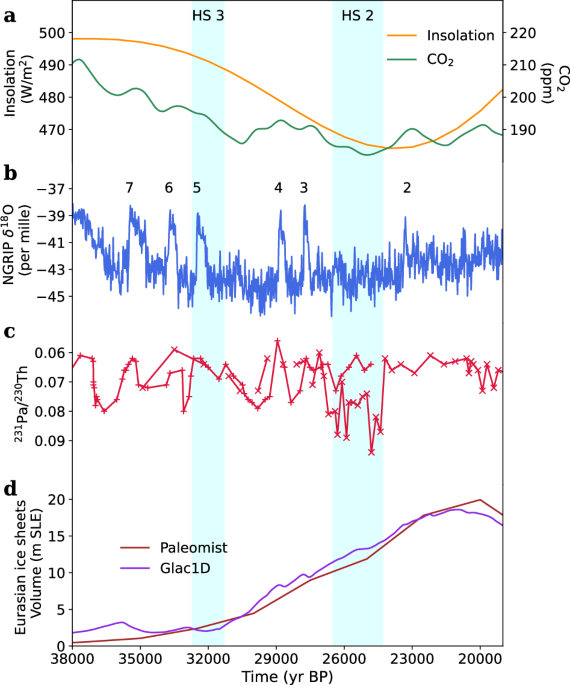
early MIS 3 (roughly around 55,000 yr BP)12. Consequently, the EIS likely underwent substantial advances after MIS 3 (Fig. 1d), ultimately reaching its maximum extent at the Last Glacial

Maximum (LGM)5,10,13,14. Accompanied by the substantial expansion of the EIS, boreal summer insolation decreased from around 35,000 yr BP, and the CO2 values remained at relatively low

levels (between 185 and 200 ppm, Fig. 1a). At the same time, the NAIS grew from an intermediate size towards the LGM. Several millennial-scale abrupt climate shifts, known as the

Dansgaard-Oeschger (DO) events, as well as Heinrich events, occurred during this period (Fig. 1b, c), with the latter associated with massive discharges of ice/freshwater into the North

Atlantic, leading to shifts between different modes of the Atlantic Meridional Overturning Circulation (AMOC)15,16,17,18. Within the timescale of glacial-interglacial cycles, the

relationship among insolation, CO2 changes, and the glaciation of the climate-cryosphere system has been extensively studied, with a particular focus on the glacial inception during MIS 5

[e.g., ref. 19]. It is widely accepted that the glacial inception arises from a bifurcation transition, where nonlinear dynamics of the climate-cryosphere system dominated19,20,21. A

logarithmic relation is proposed between the summer maximum insolation at 65∘N and the CO2 threshold for triggering glacial inception21,22. With a CO2 value of 200 ppm, an insolation value

of around 490 W/m2 or lower is needed to initiate ice sheet growth. Commonly, these glaciations refer to the Northern Hemisphere ice sheets as a whole. However, the NAIS and the EIS may

respond at different paces, as they may be influenced by distinct climate regimes. The North Atlantic current, originating in the Gulf of Mexico, transports heat eastward across the North

Atlantic and further north into the Nordic Seas. Combined with prevailing southwesterly winds across the North Atlantic, the climate in northwestern Europe (in particular Scandinavia) is

much warmer than that over North America23,24. Using an Earth system Model of Intermediate Complexity (EMIC) under transient orbital and greenhouse gases (GHGs) forcing during MIS 5,

Kageyama et al.25 illustrate that ice sheet first formed over North America, but not over Eurasia, as the latter was too temperate. Using a more complex Earth system model, Lofverstrom et

al.24 propose that the initially glaciated NAIS could block freshwater transport from the Arctic through the Canadian Archipelago, while redirecting it to the east of Greenland. This leads

to reductions in North Atlantic deep water formation over the Nordic Seas, expansions in sea ice extent and decreases in sea surface temperature, thereby promoting the inception of the EIS.

However, on the other hand, vigorous deep water formation and associated northward heat transport also bring more moisture to Eurasia, which could likewise fuel ice sheet expansion (the

so-called “Nordic heat pump”)26. The relative contributions of colder but drier conditions or warmer but more humid conditions, both potentially facilitating ice sheet growth across various

paleo time periods, have been widely discussed. During the middle Pleistocene transition, the emergence of larger EIS is proposed to be associated with the warmer North Atlantic sea surface

temperature [e.g.,refs. 27,28]. The strengthened Atlantic inflow into the Nordic Seas is also proposed to facilitate the growth of the EIS during the end of MIS 5 and the onset of the

LGM29,30,31,32. Using a complex Earth system model including atmosphere-ocean-ice sheet interactions (AWI-ESM), our study investigates the expansion behaviors of the EIS after MIS 3 under

different ocean states. The results show that the regrowth of the EIS is induced by a bifurcation transition, where a substantial thin ice sheet is initially formed before an increase in ice

volume. A weakened state of the AMOC, coupled with reduced North Atlantic deep water formation in Nordic Seas appears to be a prerequisite for the buildup of the EIS. Additionally, we

emphasize that the spatial distributions of the EIS could be highly sensitive to background temperature and precipitation changes, posing challenges to better simulate the EIS during glacial

periods. RESULTS BIFURCATION TRANSITION OF THE EIS INDUCED BY WEAKENED AMOC EVOLUTION OF THE EIS IN TRANSIENT SIMULATIONS Transient simulations with varying insolation and GHGs are

performed using the Earth system model AWI-ESM33,34. The coupling between climate and ice sheets (focusing on the entire Northern Hemisphere domain) is initialized from 38,000 yr BP, with a

climate acceleration factor of 20 applied due to computational cost (for details, see Methods). Starting at 32,000 yr BP (in the ice sheet timescale), freshwater perturbations of 0.2 Sv and

0.3 Sv are consistently applied to the Ice-rafted debris (IRD) belt to mimic different AMOC states until 20,000 yr BP (Fig. 2)35. Accordingly, the experiments are named after the initial ice

sheet dataset and the strengths of freshwater hosing (Paleomist-0.2, Paleomist-0.3). A simulation without freshwater hosing is also conducted as a reference. The main focus period of this

study is from 32,000 to 20,000 yr BP. The AMOC response to freshwater perturbations in Paleomist-0.2 is characterized by a moderate reduction of 8 Sv, decreasing to 13–14 Sv (referred to as

the moderately weak mode in our study), followed by a slow recovery to 19 Sv by 25,000 yr BP. In Paleomist-0.3, the AMOC weakens substantially (to around 3 Sv, referred to as the weak mode)

and begins to recover after 26,000 yr BP, despite the ongoing freshwater forcing (Fig. 2a). The reference simulation without freshwater hosing of the AMOC is stabilized at around 20 Sv,

which we refer to as the strong mode. Compared to experiments Paleomist-0.2 and Paleomist-0.3, the weaker AMOC state is characterized by large-scale summer cooling of more than 5 °C over the

high-latitude North Atlantic, along with extreme temperature anomalies around the coasts of the Eurasian sector of the Arctic (Fig. 2c). These anomalies are associated with weakened North

Atlantic deep water formation and an expansion of sea ice (Supplementary Fig. 1d, e). Consequently, the responses of the EIS development to different ocean states differ substantially: one

characterized by substantial ice sheet buildup over the Eurasian continent (Fig. 3e), and the other with few ice dispersed over islands in the Barents Sea and relatively high elevation areas

over Siberia (Fig. 3d). The substantial buildup of the EIS happens under the scenario with weak AMOC mode (experiment Paleomist-0.3). In this experiment, rapid ice sheet expansion happens

from around 30,000 yr BP to 27,500 yr BP (Fig. 3b, blue line; Fig. 4). After 27,500 yr BP, the ice area stabilizes, with only minor changes observed thereafter. The ice area slightly

decreases before increasing again following the recovery of the AMOC around 23,000 yr BP. More interestingly, rapid increases in ice volume occur after 28,000 yr BP, when the ice sheet

extent stabilizes, and continue until 20,000 yr BP (Fig. 3a, blue line). From the simulation, an initial thin ice sheet forms rapidly (Fig. 4), accompanied by a shift in the surface mass

balance (SMB) from negative to positive (Supplementary Fig. 2), facilitated by a strong snow/ice-albedo feedback. This process further promotes the subsequent buildup of the ice sheet, which

is reinforced by the temperature-elevation feedback as the ice sheet gains height. Similarly, in the experiment with moderately weak AMOC state (Fig. 3a–b, red lines), rapid expansion in

ice extent also happens before the large increase in ice volume. However, the ice extent expands much later and smaller compared to the experiment with the weak AMOC mode, and the ice area

begins to decrease around 24,000 yr BP. The relationship between ice volume changes and the AMOC strength from different experiments is illustrated in Fig. 5. From the figure, a bifurcation

behavior of the EIS is evident in response to changes in AMOC state. A weakened AMOC state of less than 5 Sv (in our model setup) is necessary for the initial expansion and subsequent

buildup of the EIS. However, once the ice extent reaches to certain value or the ice volume becomes considerably large, the influence of the AMOC state on changes in ice area is shown to be

minor (Figs. 2a, 3a, b). In other words, the existence of bi-stability in the EIS is evident, where two stable states can coexist under the same AMOC strength. CLIMATE AND SMB CHANGES To

better understand how different climate states influence ice sheet expansions, we compare changes in surface air temperature and precipitation, as well as changes in SMB components over

areas with substantial ice sheet buildup through time in experiment Paleomist-0.3 (Fig. 6, the selected region is indicated by the orange sector in Fig. 3e). In response to the weakening of

AMOC, both temperature and precipitation (especially in summer) decreases from 32,000 to 26,000 yr BP (Fig. 6a, b, e). Particularly at around 28,000 yr BP, summer temperature drops rapidly

from above 1 °C to below −2 °C, accompanied by large increases in summer snowfall (Fig. 6e, red and light blue lines). This leads to substantial accumulation and persistence of snow remnants

(annual minimum snow height) during the melt season, resulting in increased surface albedo (Fig. 6c, e). Consistently, the total SMB over a year increases rapidly due to the rapid reduction

of melt, while changes in total accumulation appear to be minor (Fig. 6d). After 27,000 yr BP, both precipitation and snowfall in July show a slightly decreasing trend, while the

temperature remains below −5 °C. A similar analysis is conducted for experiment Paleomist-0.2 (Supplementary Fig. 3), where mean surface air temperatures over the same region are higher than

that in experiment Paleomist-0.3. Moreover, much less snow accumulation, lower surface albedo, and stronger melting are illustrated (Supplementary Fig. 3c, d), which could prevent the

initial buildup of the EIS. Lower temperatures not only indicate less heat transport, but could also result in more snowfall rather than rainfall (when temperatures vary around 0 °C),

potentially increasing albedo and reducing melt. In our experiments, the initial expansions of the EIS are preceded by weakened AMOC-induced decreased temperature. Due to the weakening of

the AMOC, especially during summer, surface air temperatures in Fennoscandia and western Siberia drop, leading to the persistence of snowfall (Fig. 2b–d). This, in turn, increases surface

albedo and triggers the initial expansion of the EIS. Precipitation decreases over the Arctic in response to the weakened AMOC (Supplementary Fig. 1a–c), indicating that influence of

precipitation on the SMB appears to be secondary to this process. In addition, mixed layer depth related to AMOC states is also illustrated (Supplementary Fig. 1d–f). In our simulation,

although freshwater hosing of 0.2 Sv is applied over the IRD belt, Atlantic deep water formations in the Labrador Sea and the Nordic Seas remain active. With a stronger freshwater hosing of

0.3 Sv, Atlantic deep water formation in the Nordic Seas is deactivated, leading to a further southward extension of sea ice (Supplementary Fig. 1d, e). This is likely a prerequisite for the

strong cooling over Fennoscandia. SENSITIVITY OF EIS TO TEMPERATURE AND PRECIPITATION CHANGES NONLINEAR RESPONSES OF SMB TO TEMPERATURE AND PRECIPITATION To understand the nonlinear

responses in ice sheet development, we performed sensitivity experiments on the SMB (see Methods). A baseline climatology over Eurasia is first calculated (Fig. 7a, b, black lines).

Temperature and precipitation shifts are then applied to mimic conditions at different locations or perturbations within a specific location. By systematically testing these different

combinations, tipping points or thresholds where ice sheet development transitions from stable to nonlinear responses are identified. The calculated minimum snow height (Fig. 7c, shaded,

contour indicates annual mean snowfall), and total SMB over a year (Fig. 7d, shaded, contour indicates July snowfall) are illustrated, where strong non-linearity becomes evident with

variations in both temperature and precipitation. From the figure, the reference climate (brown dot) is close to a tipping point. A slight decrease in temperature or an increase in

precipitation can induce considerable remnant snow accumulation and shift the total SMB to a positive value (brown arrows). Overall, the SMB variations follow a stepped distribution. When

temperatures fall below a certain threshold (e.g., July temperature of −2 °C in the figure), changes in precipitation dominate SMB variations. At higher temperatures (e.g., 4 °C in the

figure), large negative SMB prevails. In intermediate temperature ranges, both temperature and precipitation changes can contribute to substantial SMB shifts. These large shifts in SMB/snow

heights may be related to the positive snow-albedo feedback triggered by remnants of snowfall. A similar analysis is also applied to the Paleomist-0.2 experiment, but the baseline climate in

this case is much further from a tipping point (Supplementary Fig. 4). THE HIGHLY SENSITIVE EIS BUILDUP PATTERN As is inferred from Fig. 7, the expansion of the EIS is highly sensitive to

climate changes within certain ranges: either a slight decrease in temperature or an increase in precipitation could trigger the shift (brown dot and its surroundings). The climate

variations induced by different factors (including AMOC states, atmospheric circulation or model bias) could easily encompass the most sensitive variations. In other words, small deviations

in background climates could result in substantially different patterns of the EIS. This poses greater challenges via modeling for investigating the competing effects of cold-dry and

warm-humid conditions on the evolution of the EIS (in terms of spatial pattern) across different time periods27,28,29,30,31,32. Moreover, we note that changes in orbits or atmospheric

composition could also cause a shift of the sensitive bands in SMB (Fig. 7 and Supplementary Fig. 4). DISCUSSION In this study, we investigate for the first time the development of the EIS

from MIS 3 to the LGM, using the sophisticated Earth system model AWI-ESM, which includes interactive ice sheets. The main conclusions are as follows: * 1. The EIS forms through a rapid

transition following MIS 3, with large remnants of snow cover or thin ice altering albedo in response to cooling over Eurasia. * 2. The main triggering mechanism for the rapid buildup of the

EIS is through a weakened AMOC. More specifically, the weakening of North Atlantic deep convection, along with the expansion of sea ice in the Nordic Seas, appears to play a crucial role. *

3. Sensitivity studies suggest that surface mass balance changes over the EIS could respond highly nonlinearly to variations in temperature and precipitation, highlighting the EIS’s high

sensitivity. The bifurcation transition marks the EIS buildup, with a rapid surface air temperature drop and ice expansion preceding substantial ice volume growth, underscoring the ice

sheet-climate system’s strong non-linearity. This is similar to previous studies using Earth system models of intermediate complexity (EMICs), but with a focus on glacial inception19,36,37.

However, we note that the bifurcation transition proposed in our study concerns the AMOC states within the climate system, differing from these studies that focus on orbital and GHG forcing.

In addition, our results align with other research using various reconstruction methods, such as radiocarbon-dating of moss, demonstrating the sensitivity and rapidity of ice cover

expansion38,39,40. With our model setup, despite transient decreases in insolation and GHGs, moderately weak AMOC states are still insufficient to trigger the buildup of the EIS during this

period. The main reason can be attributed to the strong heat transported to the Nordic Seas (Fig. 2b). Thus, a freshening of North Atlantic deep convection regions and the subsequent

expansion of sea ice are likely required for ice sheet development over Scandinavia. This is also observed in Talento et al.22, where considerable ice growth in Scandinavia during glacial

inception requires low CO2 conditions and is associated with weak AMOC states. Lofverstrom et al.24 focusing on glacial inception during MIS 5 suggests that the closure of Canadian Arctic

Archipelago gateways, combined with the opening of the Bering Strait could cause the freshening in Nordic Seas. Different from glacial inception during MIS 5, the size of the NAIS is

relatively large during MIS 3. Both the gateways of Canadian Arctic Archipelago and the Bering Strait are closed (Supplementary Fig. 5). However, millennial-scale abrupt shifts (DOs)

occurred, accompanied by large shifts between stadial and interstadial states, as well as changes in AMOC states (Fig. 1b, c)15. Our three AMOC states (strong, moderately weak and weak AMOC

mode) can be interpreted as being representative of interstadial, stadial and Heinrich-Stadial conditions, with the clear indication that the stronger the AMOC reduction, the more favorable

the conditions of EIS initiation once a critical slowdown of the AMOC is reached. In our simulations, this might imply that Heinrich Stadial AMOC modes are the best match. However, we expect

that the threshold itself will be different depending on the model applied. Additionally, weak AMOC conditions lead to significant forest declines and shrub expansions across Eurasia,

potentially promoting the buildup of the EIS (not shown). However, we note that although critical low temperatures are essential for the initial buildup of the EIS (via the ice-albedo

feedback), once the EIS reaches a certain size (due to the temperature-elevation feedback), a strengthened AMOC, accompanied by increased Atlantic inflow into Eurasia could enhance SMB

through increased precipitation, thus promoting further growth of the EIS (Figs. 3 and 7)32. The NAIS are also dynamically simulated, with their responses thoroughly examined in another

study, which emphasizes the importance of snow-albedo feedback, particularly in summer, for their development41. Its development is further amplified by a weak AMOC state, which contributes

to both lower surface temperatures over North America and increased moisture transport from the North Atlantic warm pool. In addition to Paleomist, we further tested another initial ice

sheet configuration with a more extensive NAIS (Glac1D, Supplementary Fig. 6a13). The responses of the simulated EIS and background climate are largely consistent with those in Paleomist

(Supplementary Figs. 6b, c and 7), indicating that the bifurcation behavior associated with AMOC states is robust. A previous study proposes that an increase in the size of the NAIS could

modify summer stationary wave field, resulting in cooling in Europe and warming in northeastern Siberia, thus induce a westward migration of the EIS42. In our model, the larger North

American ice sheets cause a slight eastward shift of the EIS (Supplementary Fig. 6), but this has a secondary impact on the EIS’s final growth. We apply climate acceleration to balance

computational limits with key considerations: it ensures an acceptable atmospheric response and upper-ocean adaptation (sufficient for modeling land-based Northern Hemisphere ice sheets),

while simultaneously allowing for the introduction of various hosing scenarios to assess the influence of ocean states on ice sheet development. However, the absence of millennial-scale

variations may shift the timing compared to geological reconstructions1. We speculate that multiple weakened AMOC episodes may lead to varying temperature cooling patterns and ice sheet

expansion, shaped by prior buildup trends. Therefore, to accurately reproduce the trajectory and timing of EIS development during this period, synchronous coupling between climate and ice

sheet components may be desired. Furthermore, a cold bias of approximately 2.5 °C over Eurasia is present in our model (Supplementary Fig. 8), which could be beneficial for ice sheet

inception and for lowering the threshold of AMOC states. The bias pattern aligns with the extent of the established EIS, supporting our conclusion of a highly sensitive EIS buildup feature.

Several open questions remain that require further investigation to fully understand the complexities of ice sheet-climate interactions. In experiment Paleomist-0.3, the AMOC recovers from

around 25,000 yr BP onward. This is a unique behavior that has not been demonstrated in previous standard hosing experiments. Nevertheless, studies using various complex Earth system models

without interactive ice sheets suggest that changes in ice sheet heights, orbits or GHGs could all induce rapid AMOC changes: Gong et al.43 proposed that higher Laurentide and Greenland ice

sheets enhance North Atlantic wind stress, strengthening the AMOC. Gradual changes in Northern Hemisphere ice sheet heights may trigger millennial-scale AMOC shifts44, while orbital-driven

insolation changes can also induce similar shifts by modulating low-latitude hydro-climate and/or high-latitude sea ice-ocean-atmosphere interactions45. And glacial-level atmospheric CO2

levels could similarly induce an oscillatory AMOC regime46. Determining which factor dominates the recovery of the AMOC is beyond the scope of the present paper, and would require

single-forcing experiments. We employed the advanced PICO scheme, which includes sub-shelf melt, to model the ice sheet-ocean interface. However, our experiments show no buildup of the

marine-based SBKIS. This may be because the scheme (same to other ocean forcing schemes) is calibrated for the present-day Antarctic ice sheet47 and appears unsuitable for the SBKIS. The

same applies to the calving laws, which are tuned based on the present-day Antarctic or Greenland ice sheets. This highlights the need for future work to develop an appropriate

parametrization configuration for the SBKIS during paleo times. Another possible reason is that the ocean mesh is fixed at 38,000 yr BP, meaning that changes in sea level (ocean depth) are

not considered. This could potentially also influence the buildup of the SBKIS. To wrap up, our study highlights the importance of ocean states in the development of continental ice sheets

and their role in driving regime shifts in Earth’s stability. We also emphasize that the spatial distributions of the EIS are highly sensitive to background climate changes, posing

challenges for accurately simulation. Beyond the influence of insolation, we underscore the complexity and non-linearity of Earth system development, particularly driven by internal

climate-ice sheet feedbacks, necessitating the development of complex models that incorporate ice sheets. METHODS MODEL DESCRIPTION The experiments in this study are conducted with a complex

Earth system model AWI-ESM (version 2.1), and the model is asynchronously coupled to the Parallel Ice Sheet Model (PISM, version 1.2). AWI-ESM includes the atmosphere and land surface

components from ECHAM6, and the sea ice-ocean component from FESOM248. ECHAM6 is the sixth generation of the General Circulation Model (GCM) ECHAM, incorporating diabatic processes and

large-scale circulations ultimately driven by radiative forcing49. Its dynamic core is based on the vorticity and divergence form of the primitive equations. The land surface model

accounting for land process changes (JSBACH) is incorporated in ECHAM6, with dynamic vegetation switched on in the simulations. The horizontal resolution is approximately 1.9° × 1.9° on a

T63 Gaussian grid, and 47 vertical levels extending up to 0.01 hPa of the atmosphere are applied. FESOM2 (Finite volumE Sea ice-Ocean Model) is formulated on an unstructured mesh to resolve

global sea ice-ocean characteristics, with multi-resolution modeling functionality50. It builds upon FESOM1.4, but uses finite-volume discretization instead of finite-element discretization.

The resolution here ranges spatially from 20 km, accounting for dynamically active regions (e.g., polar and coastal areas), to 130 km over specific open ocean (Supplementary Fig. 5). The

AWI-ESM model has been applied in paleoclimate simulations across various temporal intervals51,52. It also participates in the Paleoclimate Modeling Intercomparison Project 4 (PMIP 4) and

demonstrates performance comparable to other models53. PISM is a three-dimensional thermo-mechanically coupled ice sheet model54. It uses the hybrid shallow ice approximation (SIA) and

shallow shelf approximation (SSA) for computing the stress balance, and the enthalpy-based Glen-Paterson-Budd-Lliboutry-Duval law for ice deformation55,56,57,58. A SIA enhancement factor of

5.0 and a SSA enhancement factor of 0.5 are used. For the basal condition, a till layer is assumed, and a pseudo-plastic sliding law is applied to determine basal sliding59. The yield stress

is based on the Mohr-Coulomb criterion, with the associated friction angle depending on bed elevation: 5° below −50 m, 30° above 0 m, and linearly interpolated in between. The Lingle-Clark

scheme is used for the bedrock deformation60. At the ice shelf-ocean interface, the PICO scheme is applied47. Ice shelf calving is controlled by a combination of eigen-calving,

thickness-calving, and von Mises stress calving. The calving processes are influenced by horizontal strain rates, a threshold ice thickness of 150 m, and tensile stresses. The spatial domain

is on a Northern Hemisphere polar stereographic projection, with resolution of 20 km × 20 km. The parameter settings are tuned using a glacial index method, with LGM and PI climate outputs

from AWI-ESM, to align with reconstructed sea-level variations over the last glacial cycle61. COUPLING BETWEEN THE CLIMATE AND ICE SHEETS The model is initialized using the corresponding

initial ice sheet boundary conditions. Accordingly, a 50-year spin-up period is applied to the climate model, using the fixed 38,000 yr BP orbital parameters, GHG concentrations, and ice

sheet configurations. The atmosphere is spun-up from a cold start, as its response is relatively fast, while the ocean is spun-up from an equilibrated LGM condition. For the ice sheet

spin-up, a heuristic scheme is used to determine the temperatures at depth, taking into account ice thickness, surface temperature, surface mass balance, and geothermal flux. The temperature

is computed as the solution to a steady one-dimensional differential equation, and the vertical velocity is linearly interpolated between the surface mass balance at the top and zero at the

base. Starting at 38,000 yr BP, the fully coupled model is enabled, and the model is allowed to self-adjust to more consistent conditions across the different components until 32,000 yr BP.

Asynchronous coupling with a factor of 20 between the climate components and the ice sheets is conducted, due to the computational constraints arising from the relatively high-resolution

GCM. The AWI-ESM is first integrated with prescribed ice sheet boundaries for 5 years. The atmospheric variables (e.g., temperature, precipitation, short-wave and longwave radiation, and

cloud cover) are taken for calculating the surface mass balance (SMB) for PISM. Then the ice sheet model PISM is integrated for 100 years. Afterwards, the simulated ice sheet state is used

as new boundary condition, and the respective ice mask, orography and freshwater changes are passed back to the climate components. As such, the simulations between AWI-ESM and PISM are

switched back and forth. A notable feature for the coupling is that we apply an advanced surface mass balance scheme (diurnal Energy Balance Model, dEBM) for calculating the SMB62. It

accounts for changes in the Earth’s orbit and atmospheric composition while remaining computationally inexpensive, as it only requires monthly input. The coupling setup used here is the same

as in Niu et al.41. With this setup, fast responses of the atmosphere and upper ocean are ensured, which are essential for the land-based Northern Hemisphere ice sheets. At the same time,

different hosing scenarios are applied to investigate the influence of ocean states on the ice sheet development. We further note that the responses to vegetation feedback may also be

slightly delayed. Besides, note that the ocean bathymetry is fixed, since interactive adaption in unstructured ocean mesh is currently not applicable. EXPERIMENTAL DESIGN The experiments are

initialized from 38,000 yr BP during late-MIS 3, with transient changes in insolation and greenhouse gases (GHGs) applied to the model33,34. The initial ice sheet boundary condition is

based on a reconstructed 38,000 yr BP configuration derived from Paleomist, a Glacial Isostatic Adjustment (GIA)-based model dataset (Fig. 3c)14. Beginning at 32,000 yr BP (based on the ice

sheet timescale), freshwater perturbations of 0.2 Sv and 0.3 Sv are consistently imposed on the Ice-rafted debris (IRD) belt throughout the entire simulation period to mimic different AMOC

states (Fig. 2)35. These values fall within reasonable magnitudes when compared to reconstructions of freshwater input using different reconstruction methods (10−1 Sv) [e.g., refs. 63,64].

In our simulation, the model is perturbed from a strong AMOC state during MIS 3. However, we note that a direct, one-to-one comparison of these values to estimates from Heinrich events is

not applicable. We emphasize that the responses of AMOC states to freshwater perturbations are model-dependent. Furthermore, a reference simulation without freshwater perturbation is also

conducted. The experiments are named after the initial ice sheet datasets and the strengths of freshwater hosing (Paleomist-ref, Paleomist-0.2, Paleomist-0.3). Based on these experiments,

the responses of the EIS are investigated. To account for uncertainties related to the NAIS sizes, we also tested another initial ice sheet configuration from Glac1D13, where the North

American ice sheets are more extensive (Supplementary Fig. 6a). The same settings as in Paleomist, including freshwater hosing of 0.2 and 0.3 Sv, are applied. The results are largely similar

to those from Paleomist, suggesting that the size of NAIS has a secondary influence on the initial glaciation of the EIS. Moreover, we note that our study primarily focuses on the mechanism

responsible for glaciating the EIS, rather than on the specific trajectory or exact timing of its development. Sensitivity experiments are conducted to gain a comprehensive understanding of

the nonlinear changes in the SMB driven by variations in temperature and precipitation. A baseline monthly climatology over Eurasia is first calculated (shown in orange sector in Fig. 3e)

at approximately 28,000 yr BP using the Paleomist-0.3 experiment, corresponding to the early stages of the EIS inception. Systematic shifts in temperature and precipitation are applied, with

temperature varying from −5 to 5 °C relative to the mean, and precipitation scaled from 0% to 500% of its original values (Fig. 7a, b). All other factors remain unchanged. Based on these

adjustments, the SMB is recalculated using dEBM. The dEBM is initialized in boreal October (beginning of the hydrological year) with a 15-month spin-up period, after which the second full

cycle is analyzed62. Similarly, we also tested with experiment Paleomist-0.2, but the respective climate is much further from a tipping point due to the relative high temperature

(Supplementary Fig. 4). In this case, greater precipitation is required to achieve a positive SMB. However, the nature of the SMB response remains largely the same. DATA AVAILABILITY The

datasets used and/or analyzed during the current study are available from the corresponding author upon reasonable request. CODE AVAILABILITY All codes are available from the corresponding

author on request. REFERENCES * Clark, P. U. et al. The last glacial maximum. _Science_ 325, 710–714 (2009). Article  CAS  Google Scholar  * Hughes, A. L., Gyllencreutz, R., Lohne, Ø. S.,

Mangerud, J. & Svendsen, J. I. The last Eurasian ice sheets–a chronological database and time-slice reconstruction, DATED-1. _Boreas_ 45, 1–45 (2016). Article  Google Scholar  * Patton,

H. et al. The extreme yet transient nature of glacial erosion. _Nat. Commun._ 13, 7377 (2022). Article  CAS  Google Scholar  * Mangerud, J. et al. A Middle Weichselain ice-free period in

Western Norway: the Ålesund Interstadial. _Boreas_ 10, 447–462 (1981). Article  Google Scholar  * Arnold, N. S., van Andel, T. H. & Valen, V. Extent and dynamics of the scandinavian ice

sheet during oxygen isotope stage 3 (65,000–25,000 yr BP) 1. _Quat. Res._ 57, 38–48 (2002). Article  Google Scholar  * Wohlfarth, B. & Näslund, J.-O. Fennoscandian ice sheet in MIS

3–Introduction. _Boreas_ 39, 325–327 (2010). Article  Google Scholar  * Wohlfarth, B. Ice-free conditions in Sweden during marine oxygen isotope stage 3? _Boreas_ 39, 377–398 (2010). Article

  Google Scholar  * Mangerud, J., Gulliksen, S. & Larsen, E. 14C-dated fluctuations of the western flank of the Scandinavian Ice Sheet 45–25 kyr BP compared with Bølling–Younger Dryas

fluctuations and Dansgaard–Oeschger events in Greenland. _Boreas_ 39, 328–342 (2010). Article  Google Scholar  * Helmens, K. F. & Engels, S. Ice-free conditions in eastern Fennoscandia

during early Marine Isotope Stage 3: lacustrine records. _Boreas_ 39, 399–409 (2010). Article  Google Scholar  * Lambeck, K., Purcell, A., Zhao, J. & SVENSSON, N.-O. The Scandinavian ice

sheet: from MIS 4 to the end of the Last Glacial Maximum. _Boreas_ 39, 410–435 (2010). Article  Google Scholar  * Patton, H., Hubbard, A., Andreassen, K., Winsborrow, M. & Stroeven, A.

P. The build-up, configuration, and dynamical sensitivity of the Eurasian ice-sheet complex to Late Weichselian climatic and oceanic forcing. _Quat. Sci. Rev._ 153, 97–121 (2016). Article 

Google Scholar  * Mangerud, J. et al. Did the Eurasian ice sheets melt completely in early Marine Isotope Stage 3? New evidence from Norway and a synthesis for Eurasia. _Quat. Sci. Rev._

311, 108136 (2023). Article  Google Scholar  * Tarasov, L., Dyke, A. S., Neal, R. M. & Peltier, W. R. A data-calibrated distribution of deglacial chronologies for the North American ice

complex from glaciological modeling. _Earth Planet. Sci. Lett._ 315, 30–40 (2012). Article  Google Scholar  * Gowan, E. J. et al. A new global ice sheet reconstruction for the past 80 000

years. _Nat. Commun._ 12, 1199 (2021). Article  CAS  Google Scholar  * Dansgaard, W. et al. Evidence for general instability of past climate from a 250-kyr ice-core record. _nature_ 364,

218–220 (1993). Article  Google Scholar  * Andersen, K. K. et al. High-resolution record of Northern Hemisphere climate extending into the last interglacial period. _Nature_ 431, 147–151

(2004). Article  CAS  Google Scholar  * Lippold, J. et al. Does sedimentary 231Pa/230Th from the Bermuda rise monitor past Atlantic meridional overturning circulation? _Geophys. Res. Lett._

36, L12601 (2009). * Henry, L. G. et al. North Atlantic ocean circulation and abrupt climate change during the last glaciation. _Science_ 353, 470–474 (2016). Article  CAS  Google Scholar  *

Calov, R., Ganopolski, A., Claussen, M., Petoukhov, V. & Greve, R. Transient simulation of the last glacial inception. Part I: glacial inception as a bifurcation in the climate system.

_Clim. Dyn._ 24, 545–561 (2005). Article  Google Scholar  * Calov, R. & Ganopolski, A. Multistability and hysteresis in the climate-cryosphere system under orbital forcing. _Geophys.

Res. Lett._ 32, L21717 (2005). * Ganopolski, A., Winkelmann, R. & Schellnhuber, H. J. Critical insolation–CO2 relation for diagnosing past and future glacial inception. _Nature_ 529,

200–203 (2016). Article  CAS  Google Scholar  * Talento, S., Willeit, M. & Ganopolski, A. New estimation of critical insolation–CO2 relationship for triggering glacial inception.

_Climate_ 20, 1349–1364 (2024). Google Scholar  * Rossby, T. The North Atlantic Current and surrounding waters: at the crossroads. _Rev. Geophys._ 34, 463–481 (1996). Article  Google Scholar

  * Lofverstrom, M., Thompson, D. M., Otto-Bliesner, B. L. & Brady, E. C. The importance of Canadian Arctic Archipelago gateways for glacial expansion in Scandinavia. _Nat. Geosci._ 15,

482–488 (2022). Article  CAS  Google Scholar  * Kageyama, M., Charbit, S., Ritz, C., Khodri, M. & Ramstein, G. Quantifying ice-sheet feedbacks during the last glacial inception.

_Geophys. Res. Lett._ 31, L24203 (2004). * Hansen, B. & Østerhus, S. North Atlantic–Nordic seas exchanges. _Prog. Oceanogr._ 45, 109–208 (2000). Article  Google Scholar  * Barker, S. et

al. Strengthening Atlantic inflow across the mid-Pleistocene transition. _Paleoceanogr. Paleoclimatol._ 36, e2020PA004200 (2021). Article  Google Scholar  * Sánchez Goñi, M. F. et al. Moist

and warm conditions in Eurasia during the last glacial of the middle pleistocene transition. _Nat. Commun._ 14, 2700 (2023). Article  Google Scholar  * Ruddiman, W. & McIntyre, A. Warmth

of the subpolar North Atlantic Ocean during Northern Hemisphere ice-sheet growth. _Science_ 204, 173–175 (1979). Article  CAS  Google Scholar  * McManus, J. F., Oppo, D. W., Keigwin, L. D.,

Cullen, J. L. & Bond, G. C. Thermohaline circulation and prolonged interglacial warmth in the North Atlantic. _Quat. Res._ 58, 17–21 (2002). Article  Google Scholar  * Hebbeln, D.,

Dokken, T., Andersen, E. S., Hald, M. & Elverhøi, A. Moisture supply for northern ice-sheet growth during the Last Glacial Maximum. _Nature_ 370, 357–360 (1994). Article  Google Scholar

  * Simon, M. H. et al. Atlantic inflow and low sea-ice cover in the Nordic Seas promoted Fennoscandian Ice Sheet growth during the Last Glacial Maximum. _Commun. Earth Environ._ 4, 385

(2023). Article  Google Scholar  * Berger, A. Long-term variations of daily insolation and quaternary climatic changes. _J. Atmos. Sci._ 35, 2362–2367 (1978). Article  Google Scholar  *

Köhler, P., Nehrbass-Ahles, C., Schmitt, J., Stocker, T. F. & Fischer, H. A 156 kyr smoothed history of the atmospheric greenhouse gases CO2, CH4, and N2O and their radiative forcing.

_Earth Syst. Sci. Data_ 9, 363–387 (2017). Article  Google Scholar  * Hemming, S. R. Heinrich events: massive late Pleistocene detritus layers of the North Atlantic and their global climate

imprint. _Rev. Geophys._ 42 (2004). * Willeit, M. et al. Glacial inception through rapid ice area increase driven by albedo and vegetation feedbacks. _Climate_ 20, 597–623 (2024). Google

Scholar  * Ganopolski, A. Toward generalized Milankovitch theory (GMT). _Climate_ 20, 151–185 (2024). Google Scholar  * Ives, J. Indications of recent extensive glacierization in

North–Central Baffin Island, NWT. _J. Glaciol._ 4, 197–205 (1962). Article  Google Scholar  * Ives, J. D., Andrews, J. T. & Barry, R. G. Growth and decay of the Laurentide Ice Sheet and

comparisons with Fenno-Scandinavia. _Naturwissenschaften_ 62, 118–125 (1975). Article  Google Scholar  * Miller, G. H. et al. Moss kill dates and modeled summer temperature track episodic

snowline lowering and ice cap expansion in Arctic Canada through the Common Era. _Climate_ 19, 2341–2360 (2023). Google Scholar  * Niu, L., Knorr, G., Krebs-Kanzow, U., Gierz, P. &

Lohmann, G. Rapid Laurentide Ice Sheet growth preceding the Last Glacial Maximum due to summer snowfall. _Nat. Geosci._ 17, 440–449 (2024). Article  CAS  Google Scholar  * Liakka, J.,

Löfverström, M. & Colleoni, F. The impact of the North American glacial topography on the evolution of the Eurasian ice sheet over the last glacial cycle. _Climate_ 12, 1225–1241 (2016).

Google Scholar  * Gong, X. et al. Higher Laurentide and Greenland ice sheets strengthen the North Atlantic ocean circulation. _Clim. Dyn._ 45, 139–150 (2015). Article  Google Scholar  *

Zhang, X., Lohmann, G., Knorr, G. & Purcell, C. Abrupt glacial climate shifts controlled by ice sheet changes. _Nature_ 512, 290–294 (2014). Article  CAS  Google Scholar  * Zhang, X. et

al. Direct astronomical influence on abrupt climate variability. _Nat. Geosci._ 14, 819–826 (2021). Article  CAS  Google Scholar  * Vettoretti, G., Ditlevsen, P., Jochum, M. & Rasmussen,

S. O. Atmospheric CO2 control of spontaneous millennial-scale ice age climate oscillations. _Nat. Geosci._ 15, 300–306 (2022). Article  CAS  Google Scholar  * Reese, R., Albrecht, T.,

Mengel, M., Asay-Davis, X. & Winkelmann, R. Antarctic sub-shelf melt rates via PICO. _Cryosphere_ 12, 1969–1985 (2018). Article  Google Scholar  * Sidorenko, D. et al. Evaluation of

FESOM2. 0 coupled to ECHAM6. 3: preindustrial and HighResMIP simulations. _J. Adv. Model. Earth Syst._ 11, 3794–3815 (2019). Article  Google Scholar  * Stevens, B. et al. Atmospheric

component of the MPI-M Earth system model: ECHAM6. _J. Adv. Model. Earth Syst._ 5, 146–172 (2013). Article  Google Scholar  * Scholz, P. et al. Assessment of the Finite-volumE Sea ice-Ocean

Model (FESOM2. 0)–Part 1: description of selected key model elements and comparison to its predecessor version. _Geosci. Model Dev._ 12, 4875–4899 (2019). Article  Google Scholar  * Shi, X.,

Werner, M., Wang, Q., Yang, H. & Lohmann, G. Simulated mid-holocene and last interglacial climate using two generations of AWI-ESM. _J. Clim._ 35, 4211–4231 (2022). Article  Google

Scholar  * Hossain, A. et al. The impact of different atmospheric CO2 concentrations on large scale Miocene temperature signatures. _Paleoceanogr. Paleoclimatol._ 38, e2022PA004438 (2023).

Article  Google Scholar  * Kageyama, M. et al. The PMIP4 Last Glacial Maximum experiments: preliminary results and comparison with the PMIP3 simulations. _Climate_ 17, 1065–1089 (2021).

Google Scholar  * the PISM authors. PISM, a Parallel Ice Sheet Model https://www.pism.io (2021). * Bueler, E. & Brown, J. Shallow shelf approximation as a “sliding law” in a

thermomechanically coupled ice sheet model. _J. Geophys. Res. Solid Earth_ 114, 1–21 (2009). Article  Google Scholar  * Paterson, W. & Budd, W. Flow parameters for ice sheet modeling.

_Cold Reg. Sci. Technol._ 6, 175–177 (1982). Article  Google Scholar  * Lliboutry, L. & Duval, P. Various isotropic and anisotropic ices found in glaciers and polar ice caps and their

corresponding rheologies. In _Ann. Geophys_., 3, 207–224 (Gauthier-Villars, 1985). * Aschwanden, A., Bueler, E., Khroulev, C. & Blatter, H. An enthalpy formulation for glaciers and ice

sheets. _J. Glaciol._ 58, 441–457 (2012). Article  Google Scholar  * Cuffey, K. M. & Paterson, W. S. B. _The Physics of Glaciers_ (Academic Press, 2010). * Lingle, C. S. & Clark, J.

A. A numerical model of interactions between a marine ice sheet and the solid earth: application to a West Antarctic ice stream. _J. Geophys. Res. Oceans_ 90, 1100–1114 (1985). Article 

Google Scholar  * Niu, L., Lohmann, G., Hinck, S., Gowan, E. J. & Krebs-Kanzow, U. The sensitivity of Northern Hemisphere ice sheets to atmospheric forcing during the last glacial cycle

using PMIP3 models. _J. Glaciol._ 65, 645–661 (2019). Article  Google Scholar  * Krebs-Kanzow, U. et al. The diurnal Energy Balance Model (dEBM): a convenient surface mass balance solution

for ice sheets in Earth system modeling. _Cryosphere_ 15, 2295–2313 (2021). Article  Google Scholar  * Roche, D., Paillard, D. & Cortijo, E. Constraints on the duration and freshwater

release of Heinrich event 4 through isotope modelling. _Nature_ 432, 379–382 (2004). Article  CAS  Google Scholar  * Zhou, Y. & McManus, J. F. Heinrich event ice discharge and the fate

of the Atlantic Meridional Overturning Circulation. _Science_ 384, 983–986 (2024). Article  CAS  Google Scholar  Download references ACKNOWLEDGEMENTS This study is supported by the German

Federal Ministry of Education and Research (BMBF) funded project PalMod (grant numbers 01LP1915A and 01LP2303A to G.K. and 01LP1916B and 01LP2313A to G.L.) and contributes to the Helmholtz

research program “Changing Earth—Sustaining our Future” and the Helmholtz Climate Initiative “REKLIM”. This work is also supported by the ERC grant “i2B” (grant no. 101118519), funded by the

European Union. U.K.-K. is supported by the Deutsche Forschungsgemeinschaft (Excellence Cluster “EXC 2077: The Ocean Floor - Earth’s Uncharted Interface”, project no. 390741603). The

development of PISM is supported by NASA grant NNX17AG65G and NSF grants PLR-1603799 and PLR-1644277. We thank the Max-Planck Institute in Hamburg and colleagues from the AWI for making

ECHAM6-JSBACH and FESOM2 available. Computational resources were made available by the infrastructure and support of the computing center of the AWI in Bremerhaven and the DKRZ in Hamburg,

Germany. FUNDING Open Access funding enabled and organized by Projekt DEAL. AUTHOR INFORMATION AUTHORS AND AFFILIATIONS * Alfred-Wegener-Institut, Helmholtz-Zentrum für Polar und

Meeresforschung, Bremerhaven, Bremen, Germany Lu Niu, Gregor Knorr, Lars Ackermann, Uta Krebs-Kanzow & Gerrit Lohmann Authors * Lu Niu View author publications You can also search for

this author inPubMed Google Scholar * Gregor Knorr View author publications You can also search for this author inPubMed Google Scholar * Lars Ackermann View author publications You can also

search for this author inPubMed Google Scholar * Uta Krebs-Kanzow View author publications You can also search for this author inPubMed Google Scholar * Gerrit Lohmann View author

publications You can also search for this author inPubMed Google Scholar CONTRIBUTIONS L.N. and G.K. designed the work. L.N. performed the Earth system modeling experiments, the analysis and

wrote the paper. L.A. helped with the Earth system modeling. L.N., G.K., U.K.-K., and G.L. contributed to the interpretation and discussion of the results. All authors provided input to the

final version of the manuscript. CORRESPONDING AUTHOR Correspondence to Lu Niu. ETHICS DECLARATIONS COMPETING INTERESTS The authors declare no competing interests. ADDITIONAL INFORMATION

PUBLISHER’S NOTE Springer Nature remains neutral with regard to jurisdictional claims in published maps and institutional affiliations. SUPPLEMENTARY INFORMATION SUPPLEMENTARY INFORMATION

RIGHTS AND PERMISSIONS OPEN ACCESS This article is licensed under a Creative Commons Attribution 4.0 International License, which permits use, sharing, adaptation, distribution and

reproduction in any medium or format, as long as you give appropriate credit to the original author(s) and the source, provide a link to the Creative Commons licence, and indicate if changes

were made. The images or other third party material in this article are included in the article’s Creative Commons licence, unless indicated otherwise in a credit line to the material. If

material is not included in the article’s Creative Commons licence and your intended use is not permitted by statutory regulation or exceeds the permitted use, you will need to obtain

permission directly from the copyright holder. To view a copy of this licence, visit http://creativecommons.org/licenses/by/4.0/. Reprints and permissions ABOUT THIS ARTICLE CITE THIS

ARTICLE Niu, L., Knorr, G., Ackermann, L. _et al._ Eurasian ice sheet formation promoted by weak AMOC following MIS 3. _npj Clim Atmos Sci_ 8, 85 (2025).

https://doi.org/10.1038/s41612-025-00982-5 Download citation * Received: 18 June 2024 * Accepted: 17 February 2025 * Published: 02 March 2025 * DOI:

https://doi.org/10.1038/s41612-025-00982-5 SHARE THIS ARTICLE Anyone you share the following link with will be able to read this content: Get shareable link Sorry, a shareable link is not

currently available for this article. Copy to clipboard Provided by the Springer Nature SharedIt content-sharing initiative