Observationally constrained global NOx and CO emissions variability reveals sources which contribute significantly to CO2 emissions

Download PDF Article Open access Published: 04 March 2025 Observationally constrained global NOx and CO emissions variability reveals sources which contribute significantly to CO2 emissions

Shuo Wang1,2, Jason Blake Cohen1,3, Luoyao Guan1,3, Lingxiao Lu1,3, Pravash Tiwari1,3 & …Kai Qin1,3 Show authors npj Climate and Atmospheric Science volume 8, Article number: 87 (2025) Cite

this article

1597 Accesses

10 Altmetric

Metrics details

Global high-resolution emission inventories of trace gases require refinement to align with ground-based observations, especially for extreme events and changing sources. This study utilizes

two satellites to globally quantify NO2 and CO concentrations on daily to weekly scales and estimate emissions with uncertainty bounds, grid-by-grid, for regions with significant

variability in 2010. These emissions demonstrate overall increased emissions and identify missing sources compared with various inventories. The NOx and CO emissions are 5.76 × 105–6.25 ×

106 Mt/yr and 1.06 × 107–2.78 × 107 Mt/yr, representing a mean 200% and 130% increase. Significant emissions originate from typical and atypical sources, exhibiting short-to-medium-term

variability, primarily driven by biomass burning and anthropogenic activities, with substantial redistribution and compression due to long-range transport. The extra CO emissions chemically

decay into CO2, resulting in an increase in CO2 mass equivalent to 3.5% of CO2 emissions from Central Africa and 6.1% from Amazon, reflecting the importance of addressing CO from biomass

burning.

November 2021 Global fine-scale changes in ambient NO2 during COVID-19 lockdowns Article Open access 19 January 2022 Gridded fossil CO2 emissions and related O2 combustion consistent with

national inventories 1959–2018 Article Open access 07 January 2021 Introduction

There has been a significant amount of research into trace gas assessment due to the various impacts that these have on the atmospheric environment1,2, ecosystems3, climate change4 and even

human health5,6. Previous studies have made substantial advancements in constraining emissions with various spatial and temporal resolutions7,8,9,10. However, there remains a need for

approaches that incorporate high-resolution satellite data to achieve more accurate geospatial assessments of emission intensities across diverse regions. While there is a sufficient amount

of work to evaluate well-known urban, industrial, and transport sources and large and clearly identified fires in areas that have access to many measurements, there are still many gaps in

the Global South where measurements are sparse, and in regions throughout the world which are undergoing rapid economic, political, industrial, pandemic, and environmental changes11,12.

Precisely quantifying rapid changes in the temporal and spatial distribution of emissions is critical for evaluating extreme events. Neglecting these variations and relying only on long-term

average values can introduce significant biases in calculations related to the atmospheric energy budget13, radiative forcing14, cloud cover15, rainfall formation16, and pollution event

exceedances17.

Present emission inventories used by atmospheric and environmental communities for global, mesoscale, and local models, as well as for evaluating climate impacts and radiative forcing, are

mostly built using bottom-up approaches. These inventories include both anthropogenic sources, such as EDGAR (Emissions Database for Global Atmospheric Research) and MEIC (Multi-resolution

Emission Inventory for China), and fire emission source, such as FINN (The Fire Inventory from NCAR) and GFED (Global Fire Emissions Database)18,19,20. They are constructed based on

differing methodologies, which all rely heavily on statistical data and information of emissions factors, fuel consumed, etc. The fire-based emissions products also include some indirect

satellite-derived data of fire activity or land cover change. However, all of these emissions datasets are not based on directly observed concentrations or columns of NOx or CO. These

methods often struggle to identify sudden pollution events in areas without any a priori source information, particularly in regions experiencing rapid changes or unexpected events8. Given

the rapid changes in the climate, it has been repeatedly demonstrated that the bottom-up approach is not the best way to model and understand many significant atmospheric events.

Top-down studies have been used and found to be effective for very-long-lived species, such as N2O (Nitrous Oxide) and CH4 (Methane), and CFCs (Chlorofluorocarbons)21,22. Top-down approaches

for NOx (Nitrogen Oxides) and CO (Carbon Monoxide) require knowledge of the atmospheric column at high spatial and temporal resolution1,2, due to the fact that they are not well mixed

throughout the troposphere. With appropriate observational data and knowledge of the first-order sources and sinks, the top-down approaches for shorter-lived species with lifetimes similar

to NOx (Nitrogen Oxides) and CO (Carbon Monoxide) can be effectively performed, as demonstrated in this work. However, the observations require sufficient robustness to quantify and bound

their uncertainty so that the signal can be differentiated from noise. While ground-based measurements, such as those from AERONET (for BC)23, TCCON (for CO) and Max-DOAS (for NO2)24,25,26,

can enhance local emission estimates by providing higher quality data, their effects are limited by their low spatial density. There are recent direct scaling and 3D/4DVar approaches27,28

for NO2 (Nitrogen Dioxide) and AOD (Aerosol Optical Depth) that have shown improvements in capturing time series of known pollution events, such as urban air pollution episodes and wildfire

emissions, although these methods have also been shown to frequently lead to spatial-temporal mismatches1. However, these methods often struggle to identify sudden pollution events in areas

without any a priori source information, particularly in regions experiencing rapid changes or unexpected events29,30. Other studies have focused on Kalman Filters or other more advanced

assimilation methods, which face challenges due to the need to quantify uncertainties in observational data and model parameters, factors that are often difficult to determine precisely31.

While there are existing global-scale studies that have used top-down methods to constrain NO2 and CO emissions32,33,34,35,36,37, these studies are based on models that are not always

available for public use and when accessible are hard to change or modify, produce results at lower spatial and/or temporal resolution, are not readily adapted to suit local emissions and

environmental conditions or policies, and frequently make scientific assumptions about emissions ratios of NO to NO2, as well as NOx to CO. This work emphasizes a more flexible and

accessible framework that can be broadly utilized by both scientific and applied communities, and across greater environmental and emissions conditions and standards.

NOx and CO are two key factors in emission inventories related to ozone prediction, acid rain, carbon balance, hydroxyl (OH) radical and its impacts on the field of atmospheric chemistry,

secondary aerosol formation, and both ecosystem and human health effects32. Compared with the pre-industrial period, CO emissions have increased 2 or 3 times38, especially for biomass

burning (from 47 to 99 Tg CO per year)2. For the Southern Hemisphere, CO emission has increased 2 times than before but still has a significant uncertainty34, and the total emission for

mainland China, including unknown sources based on TROPOMI (Tropospheric Monitoring Instrument) products, is 24.75 ± 5.98 Tg NO2 per year39. However, some studies using satellite data have

found that CO emissions have been on a downward trend in recent years, while NOx emissions have not been stable, with some showing a large increase in Asia10,40, and others localized

decreases also in Asia.

This work aims to construct a newly constrained emission inventory based on direct measurements of remotely sensed columns of trace gases (NO2 and CO) using a model-free, mass-conserving

framework. The overall equation is based on a simple representation of physics, chemistry, dynamics, and in situ processing, all constrained together by the measured profiles. This method

explicitly considers the ratios between NO, NO2, and CO, therefore better accounting for the overall oxidative properties of the atmosphere where the emissions occur. Although challenges

with vertical profile differences are unavoidable, the NO2 to CO ratio serves as an effective indicator in biomass-burning regions, providing improved representation when both gases are

analyzed together1. Furthermore, this process calibrates the underlying model components across a wide range of emission magnitudes, source types, wind speeds, and UV radiation conditions by

finding the smallest possible error in terms of the underlying partial differential equations, which still allows for effectively sampling the breadth of in situ atmospheric conditions.

This process makes the simpler modeling approach used herein more representative and flexible than traditional models, which may not be calibrated for local conditions or under extreme

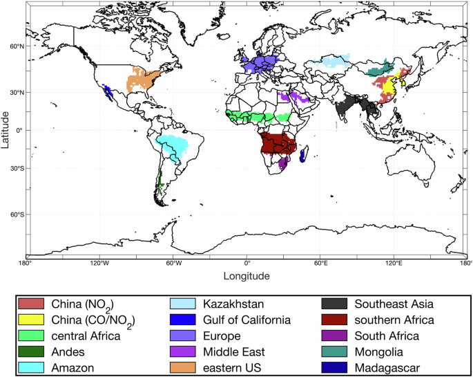
events.

The regions include emissions from biomass-burning sources (Amazon, Southeast Asia, central Africa, and southern Africa), urban sources (eastern US, China (CO/NO2), Europe), and industrial

and energy-related sources (China (NO2) and South Africa), as given in Fig. 1. The resulting time series exhibit both highly recurring patterns in time (biomass burning dominant) as well as

random time patterns (urban, industrial, and high wind variability dominant). A good match is found between the climatological observed column concentrations over the respective SVD regions

and the PCs over all four types (positive and negative of NO2 and CO), as given in Fig. S2. The climatological mean and standard deviation of the spatial distributions of observed NO2 and CO

after filtering are displayed in Fig. S3. The mean and standard deviation of remotely sensed NO2 and CO measurements compare reasonably well with both the merged emissions a priori from

existing inventories (Fig. S1) and SVD1 results in terms of geographic distribution.

Geographic distribution of all 15 subregions derived from SVD1 including positive and negative of NO2 and CO geographical decomposition signal.

SVD1 defines 15 unique geographic regions (Table 1) which include 76.5% of a prior NO2 emission and 89.4% of a prior CO emission. Some high-emission pixels, particularly those associated

with stable sources (e.g., continuous industrial emissions) or pixels affected by data gaps or data quality issues, are not fully captured in our statistical approach. This approach is

designed to be unbiased toward the location, timing, and type of emissions. Furthermore, certain highly episodic long-range transport events that do not contribute sufficiently to the

overall emissions variability across the 11-year dataset may also be excluded from SVD1.

column, [molecule/cm2, ×1015]), only over emission pixels (second column, [molecule/cm2, ×1015]), measured column loadings of MOPITT CO over each entire subregion (third column,

[molecule/cm2, ×1018]), only over emission pixels (fourth column, [molecule/cm2, ×1018])Full size table

The relationship between emissions and satellite observed column concentration is computed via Eqs. (1) and (2). While, in general, regions with larger emissions have a larger mean observed

column loading, this pattern does not exist everywhere, with contributions from meteorological conditions, source thermodynamics, and in situ processing also contributing. Across all

regions, significant variations in the NO2 to CO ratio are observed, likely due to the combined effects of regional differences in emission source types, the influence of different

atmospheric aging on the species, varying upwind conditions, and varying different spatial loadings. In the first case, it is known that NOx emissions are strongly related to the temperature

of combustion, while CO is related partially to combustion temperature, as well as the total amount of fuel or biomass combusted. In the second case, it is known that the atmospheric

chemical lifetime of CO is longer than that of NOx. The third case acknowledges that upwind conditions may themselves also have significant amounts of emissions. The overall mixture of each

of these three driving factors all play a role in the observed ratio of NO2 to CO, as shown in Fig. S4.

In different regions, there are significant differences observed in the underlying thermodynamics, first-order atmospheric loss, and transport terms, including regions that have a similar

level of economic development. This is consistent with environmental factors and anthropogenic drivers both contributing (i.e., climate, weather, type and location of local emissions source,

duration of emissions, geography, UV radiation and temperature), creating a different set of underlying driving factors compared with bottom-up emissions approaches.

PDFs of the best-fit value of \({a}_{1}\), \({a}_{2}\), \({a}_{3p}\) and \({a}_{3n}\) of NO2 are shown in Fig. 2, and demonstrate consistency with conditions expected in different source

regions, allowing for results that are based on the local conditions and can therefore be used to improve existing bottom-up approaches or approach top-down approaches in a consistent

manner. The range of coefficients is given across the 10th, 30th, 50th, 70th and 90th percentiles as a means to understand the range of variability of the underlying forcing terms. On a

global basis, the respective values of \({a}_{1}\) are 1.4, 2.4, 4.1, 8.5, 24.0, while the values in the Amazon and central Africa are 2.0, 4.6, 10.0, 18.3, 36.8 and 1.4, 2.2, 3.4, 5.9,

13.7, respectively, demonstrating a closer agreement with the small number of observations available than existing modeling studies12,39.

analysis of MCMFE NOx parameters over representative regions.

PDF analysis of \({a}_{1}\), \({a}_{2}[{hours}]\), \({a}_{3{\rm{n}}}[{km}]\), and \({a}_{3{\rm{p}}}[{km}]\) of MCMFE NOx over representative regions from SVD1, red line represents the

coefficients for each region, and the blue line represents all global coefficients, a Amazon; b central Africa; c China (NO2); d South Africa; e southern Africa; f Southeast Asia.

size image

There are significant differences observed between \({a}_{1}\) in the Amazon and in Southeast Asia, although both are considered clean during their respective non-biomass-burning seasons and

driven by biomass burning of native and secondary forests41. One possible explanation for this is given by the temperature at which combustion occurs, with a critical transition occurring

around 1200 °C42. This finding is consistent with work demonstrating that the Amazon may have large amounts of co-emitted methane from the stems of floodplain trees43, which would allow the

net combustion temperature of methane plus wood to exceed this threshold44, while the combustion of pure wood in Southeast Asia does not. The findings are both further supported by the fact

that \({a}_{1}\) in the Amazon is higher than some industrial areas, and second by the more frequent pyro-convection in the Amazon compared with Southeast Asia.

Central Africa is different from other biomass-burning areas due to a broad mixture of sources (anthropogenic, small industrial, grass burning, biomass burning, and forest burning), making

it difficult to identify a single value of \({a}_{1}\) on a single day across the region. The resulting distribution is due to the high amount of variability on a grid-by-grid and day-by-day

basis, and the statistics of \({a}_{1}\) being similar overall to the global value herein. Southern Africa, on the other hand, is slightly lower due to a mixture of less grass and other

low-temperature fires and a greater amount of industry and urbanization.

Another interesting point is that the region China (NO2) is found to be lower than global values, which reflects two significant changes. First, the majority of sources are from industry,

vehicles and residential sources, and second, this is a signal of increasing energy efficiency with lower efficiency combustion sources being phased out for higher energy efficiency45. The

region of China with the largest amount of variability in the ratio of NOx to NO2 is observed in the far western, energy-intensive areas, which have been undergoing considerable transition

in terms of observed absorbing aerosols over the same timeframe46, indicating efforts to reduce emissions overall and improve environmental standards.

The coefficient \({a}_{2}\) represents the lifetime of NO2, typically ranging from a few hours to several dozen hours, primarily influenced by geographical location and emission source

characteristics. Globally, the 10th, 30th, 50th, 70th and 90th percentiles of \({a}_{2}\) are 3.0, 7.6, 13.1, 21.4, and 36.3 h, respectively. In the Amazon and China (NO2), these percentiles

are 1.6, 4.8, 9.3, 15.7, 32.4, and 36.8 h, and 4.8, 10.7, 17.7, 28.6, and 37.3 h, respectively. The lifetime of NO2 is notably shorter in biomass-burning regions compared to others, with a

majority of \({a}_{2}\) values falling below 20 h. This is consistent with the general lifetime being shorter due to due to more rapid oxidation and uptake of NO2 onto co-emitted particles

in biomass-burning regions. It is also consistent with the higher plume-rise heights observed in these regions, which leads to increased overall dispersion into the third dimension,

especially so when it rises above into the generally cleaner free troposphere. This term is consistent with both chemical loss due to OH, photolysis, mixing into less polluted air, and

transfer/oxidation from the gas phase into nitrogen-based particulate matter. Therefore, regions with a lower \({a}_{2}\) generally are those that have a greater impact of nitrogen on the

behavior and distribution of NO2 in the atmosphere and climate.

The coefficient of both \({a}_{3n}\) and \({a}_{3p}\) represent the net transport out of and into the region of interest, respectively. Due to the shorter lifetime of NO2, the overall

transport is expected to be shorter than CO when co-emitted at the same place and time. The 10th, 30th, 50th, 70th and 90th percentiles of \({a}_{3n}\) and \({a}_{3p}\) are −77.9, −23.9,

−11.5, −5.6, −1.9 km and 1.9, 6.1, 11.9, 24.5, 73.9 km, respectively.

The five percentile values of \({b}_{1}\) show a notable difference between global and Amazon regions, with values of −136.7, −56.5, −30.6, −17.2, −6.7 h for the global dataset, and −82.0,

−35.4, −22.0, −11.5, −3.6 h for the Amazon, respectively. However, in specific areas with diverse emission sources like southern Africa, the five percentile values are −144.1, −62.4, −34.3,

−19.5, and −9.2 h, showing a distribution of \({b}_{2}\) that is highly consistent with global patterns.

There are two important findings related to transport distance, as observed for both NOx and CO. First, the transport distance of biomass-burning regions (Amazon, Southeast Asia, etc.) has a

lower value than other classifications (urban, industrial, and mixed), consistent with the more rapid removal of NOx on the surfaces of co-emitted aerosols and faster chemical loss due to

more concentrated emissions. Also observed is the decay around the edges of plumes in the middle troposphere being faster than near the surface, due to the lower background concentrations47.

Second, in China (CO/NO2), China (NO2), and the eastern US, even though these have large local sources, there is still a net import of NOx from other regions of the world, a factor only

previously considered in idealized studies13, or in terms of rare long-range transport events1. This implies that long-range transport of moderate pollution events may be more important than

the global modeling community is currently about to capture. Europe, on the other hand, is still found to be a region of net emissions export.

The range of variation for \({b}_{1}\) indicates significant uncertainty in global CO emissions, with values spanning from 0.5 to 1.3 (Fig. 3). In specific, higher values are observed in

China (NO2) and South Africa. One possible reason is that both regions have high amounts of atmospheric oxidation potential due to their large industrial bases, coupled with large amounts of

natural and anthropogenic VOCs, leading to considerable rapid secondary production of CO13. A second reason for this is related to sensor accuracy under high CO conditions48, due to a

combination of reduced radiance in and around the 2300 nm waveband due to high cloud coverage, high AOD, and rising global methane (also retrieved in the same waveband)49. This is consistent

with the fact that both regions have large amounts of diverse aerosol sources due to industry and have large coast lines allowing for intermittent thick cloud cover. Additionally, in South

Africa, there is also a period of the year when upwind biomass burning from other areas transports CO into the region, during which it may be of a similar order of magnitude to the local

urban and industrial sources.

PDF analysis of \({b}_{1}\), \({b}_{2}[{hours}]\), \({b}_{3{\rm{n}}}[{km}]\), and \({b}_{3{\rm{p}}}[{km}]\) of MCMFE CO over representative regions from SVD1, red line represents the

coefficients for each region, and the blue line represents all global coefficients, a Amazon; b central Africa; c China (NO2); d South Africa; e southern Africa; f Southeast Asia.

size image

Additionally, due to its longer lifetime, CO is observed to be transported further, as observed in the magnitude and distribution of coefficient \({b}_{3}\). The net input and net output are

generally consistent across all six regions in Fig. 3, but in the Amazon region, the dynamic transport shows less significance in the MCMFE model, whereas in South Africa, it plays a more

significant role. This difference can be attributed to the fact that the Amazon dataset covers late August to early November, a period of weak monsoon activity, while the location of South

Africa at the southernmost tip of Africa is exposed to stronger sea breezes during the same time period. This physical difference leads to a difference in the MCMFE-based coefficient

derivation during these specific times in these specific regions.

The retrieved NOx and CO emissions shown in Figs. 4 and 5 represent intensities tied to specific coefficients derived from the SVD analysis, capturing temporal variations across different

local times of the year in each region. These results reflect the dynamic nature of emissions influenced by local geographic, meteorological, and source-related factors. Standard deviations,

indicating emission variability, are provided in Figs. S5 and S6 for additional clarity. The different coefficients (10th through 90th percentile) correspond to different local times of the

year in each region. Based on this perspective, biomass-burning regions exhibit significant differences during different times of the year. In the Amazon and Southeast Asia, the NOx

emissions on the 10th are both high, while one is also high on the 30th and the other on the 50th consistent with50,51. South Africa exhibits a peak on the 90th, due to a mixture of local

and transported biomass burning. The mostly urban regions are more stable throughout the year compared with biomass burning, although there are still differences across the percentiles.

First, the timings of the extreme peak values in the biomass-burning areas are consistent with individual findings on the ground of when these fires occur, and their overall duration52.

Second, the emissions during non-peak times will be lower than or similar to current emission inventories, while the values during peak times will always be much higher. This is due to the

fact that most inventories currently in use today are produced using low temporal resolution data, and they are not able to capture the magnitude of extreme events as well41. Another factor

is that existing inventories tend to overestimate known individual large sources while ignoring or not addressing a larger number of small sources. Although the grid-by-grid approach in this

study identifies emissions in regions such as the Middle East, Northwest China, and Australian mining areas, these regions were excluded from the primary analysis due to their relatively

smaller scale and insufficient data to yield robust MCMFE results. It is hoped that additional remote sensing products in the future will allow successful emissions inversions over these

regions as consistent with53.

Mean of MCMFE NOx emissions with different percentiles coefficients based on the merged a priori emissions and MCMFE in 2010 [µg · (m−2 · s−1)]. a The 10th percentile; b the 30th percentile;

c the 50th percentile; d the 70th percentile; e the 90th percentile.

Mean of MCMFE NOx emissions with different percentiles coefficients based on the merged a priori emissions and MCMFE in 2010 [µg · (m−2 · s−1)]. a The 10th percentile; b the 30th percentile;

c the 50th percentile; d the 70th percentile; e the 90th percentile.

The findings with respect to CO emissions are somewhat similar to those with NOx emissions in terms of timing of the peaks when analyzing the results over different biomass-burning areas. In

these areas, the major differences are related to the ratio, which is different in each biomass-burning area, which reflects the different combustion sources and conditions. In contrast to

NOx, the CO emissions observed in industrial areas are found to have a higher value than most a priori studies, indicating that assumptions of highly efficient use of coal into a final CO2

end product may not actually occur on the ground42. The relatively temporally constant CO emissions in these regions, as compared with biomass burning and urban regions, may require further

work trained more locally to fully capture these persistent emissions, indicating that the results herein, although already larger than existing inventories, still yield an underestimate in

these regions.

The MCMFE results and a priori inventories for NOx and CO at each percentile are shown in Table 2 and Table 3. In terms of NOx, the temporal minimum of emissions is observed in Europe (1% of

current inventory) while the temporal maximum is observed in the Amazon (15.1 times current inventory), with an average across all regions of about 2.56 times of the priori dataset. The

emissions results based on the MCMFE model in China (CO/NO2) are much lower than current inventories, consistent with the fact that the region is normally heavily polluted, and the extremes

observed by the MCMFE method are, in fact, the smaller number of very clean days. In terms of CO emissions, the total emissions in China (CO/NO2) inversion are the lowest (8% of current

inventory), while the temporal maximum is observed in Central Africa (12.6 times of the emission priori), with an average of 2.36 times the global inventory, and the time series of MCMFE and

the priori emissions comparison in different regions over time are shown in Fig. S7 (NOx) and Fig. S8 (CO).

the first column being a merged priori emissions [Mt/yr] and the 2nd–6th columns are MCMFE emissions [Mt/yr] with the different percentile coefficientsFull size tableTable 3 Statistical of

total CO emissions for different regions in 2010, with the first column being a merged priori emissions [Mt/yr] and the 2nd–6th columns are MCMFE emissions [Mt/yr] with the different

percentiles’ coefficients, the 7th column is the total CO2 emissions from EDGAR in 2010Full size tableEstimation of additional CO2 production via CO oxidation

In the atmospheric environment, all emitted CO is fully oxidized to CO2 by OH. In addition, as the largest sink of OH, changes in CO also have indirect effects on the lifetime of methane and

ozone, which further impact radiative forcing, although these indirect effects are not further considered herein54,55,56. In comparison with EDGAR CO2 emissions (Table 3), the increase in

CO emissions in Amazon and Central Africa, when chemically converted into CO2 in situ, has a statistically significant impact on the actual CO2 emissions. This value has a maximum temporal

increase as high as 22.% and 10.% respectively, and an annual increase of 6.1% and 3.5%, respectively. CO in other regions also has an impact on CO2 emissions, although the value is found to

be under 1%, except for, as noted, the fact that industrial sources are underestimated in this work. This finding, we hope, will help the community address the assessment as to why there

are still large uncertainties in both the loadings of CO2 and longwave radiative forcing.

Nitrogen dioxide (NO2) and Carbon Monoxide (CO) are important due to their contributions to atmospheric oxidation and methane, as well as aerosol formation and growth. The current generation

of emissions estimations from both bottom-up and large-scale averaged top-down and approaches do not provide a sufficiently accurate, robust, and precise assessment of rapidly changing or

extreme emissions events in both space and time. This work employed a first-order model-free, mass-conserving equation, using day-by-day and grid-by-grid observations from OMI and MOPITT and

underlying properties of the environment in an unbiased manner to derive and attribute global emissions of NOx and CO due to extreme events or regions undergoing significant change, the

cases in which current emissions inventories are currently most uncertain.

This work identifies 15 regions globally and classifies them into urban, industrial, biomass burning, mixed, and long-range transport types, consistent with their different properties in

terms of emissions thermodynamics, first-order atmospheric loss, and long-range transport. Biomass-burning areas are found to have a higher amount of NO and shorter lifetime and a wider

range of transport distances compared with the other regions, consistent with co-emitted heat inducing a rise of emissions into the middle atmosphere. Atmospheric transport is also observed

to relate to physical geography, meteorology, precipitation, time of year, and source type, allowing identification of mixed source types. Furthermore, the results show that classifying

emitting regions into developed and developing economies is insufficient, with differences observed between the USA and EU, as well as industrial regions in Northern and Central China.

The results yield an inventory that captures both geographical and temporal variability uniformly for NOx and CO with medium confidence. Emissions are captured with medium to low confidence

in regions with a previously identified source type but incorrect timing (i.e., where the timing of emissions is lagged from the database) or duration of the peak event (i.e., the center of

the inventory’s timing is correct, but its duration is wrong), where both changes in driving factors over space and time, and downwind plume transport are identified as underlying reasons.

There is also a significant amount of emissions analyzed to occur outside of urban areas, which is subsequently advected into urban regions, a phenomenon which has been discussed in

idealized studies, but is not consistently found in observational studies and presently is not included in most modeling studies, which assume clean upwind conditions.

Due to its chemical transformation in situ into CO2, the resulting significant changes in CO emissions from biomass-burning areas yield significant changes in the net country-by-country CO2

emissions over some countries studied. The impacts on the national reported CO2 range from −5% to 21.5% of CO2 emitted in the respective regions based on the time of the year. This net

change may lead to additional erroneous estimates of direct global radiative forcing, as well as further indirect effects due to the impact of CO on atmospheric oxidation and methane, which

are not discussed herein.

The work then uses CO observations from MOPITT (Measurement of Pollution in the Troposphere) and NO2 observations from OMI (Ozone Monitoring Instrument), in combination with mass conserving

equations, reanalysis meteorology, and both urban and biomass burning a priori emissions data to produce a grid-by-grid and day-by-day (NOx) and week-by-week (CO) global emissions products.

These products illustrate the spatial distribution of the sources that contribute to the changes in emissions around the globe and include: industrialization, energy, transportation,

residential, biomass burning, forest fires, and mixed types8,47. For China, a priori emissions are from the combination of FINN (biomass burning) and MEIC (anthropogenic) while for other

regions, FINN is coupled with EDGAR (anthropogenic). This process quantifies the contributions of physical, chemical, and long-range transport effects, using remotely sensed observations to

generate a new optimized, long-term, high-resolution emissions inventory and uncertainty range.

The OMI on the NASA Aura satellite observes in the near-ultraviolet/visible spectrum with a 13 × 24 km2 coverage57,58 and has a ~1:30 p.m. local overpass time. OMI has been used to monitor

various atmospheric trace gases in the troposphere, including total column NO2. In this study, we use OMI Level 3 NO2 data from 2006 to 2016. To ensure data quality, screening is performed

to ensure cloud coverage is less than 30% and QA (Quality Assurance) larger than 75%. The NO2 observations are linearly interpolated onto a 0.1° × 0.1° grid.

Since there is no way to directly observe NO, assumptions are made based on the pseudo-steady-state assumption to link NO to NO239. In the boundary layer, NOx is short-lived, with a lifetime

under 1 day, which rises to up to 3 days when injected directly into the free troposphere due to biomass burning1,59. Recent studies have utilized column measurements of NO2 from OMI and

TROPOMI to constrain NOx emissions, making strong assumptions regarding the NO to NO2 ratio. These studies focus on specific geospatial domains, using well-validated a priori measurements

and detailed knowledge of local conditions, particularly in urban60, energy-intensive9, and strongly biomass-burning regions61. While there have been top-down studies using OMI and TROPOMI

data to constrain NOx emissions in various global regions, including North America and Europe, much of the detailed high-resolution analysis remains focused on Asia62,63. Furthermore, there

are very few global studies that provide daily or weekly top-down emissions at high resolution. It is expected that due to variations in emission magnitudes, technological and industrial

levels, and local environmental conditions, the assumptions applied will need to be adjusted to accurately reflect the characteristics of emissions sources in different parts of the world

and during times of the year.

MOPITT on the NASA Terra satellite detects concentrations of CO in the NIR (Near-infrared Radiation) and FIR (Far-infrared Radiation) regions and has a ~10:30 a.m. local overpass time64. The

data used herein is observed twice daily (day and night) at 1° × 1°, with measurements from 2006 to 2016, and interpolated into 0.1° × 0.1° resolution (Version 8, level 3, TIR

(Thermal-infrared radiation) + NIR, daytime).

MEIC is a high-resolution inventory of anthropogenic air pollutants and carbon dioxide emissions in China, covering more than 700 anthropogenic emission sources including SO2 (Sulfur

dioxide), NOx, CO, NMVOCs (Non-methane volatile organic compounds), NH3 (Ammonia), PM2.5, PM10, BC (Black carbon), OC (Organic carbon) and CO265,66. This work uses NOx and CO emission data

from V1.3. This data is then linearly interpolated from 0.25° × 0.25° to 0.1° × 0.1° resolution.

EDGAR is a European Commission database providing global past and present anthropogenic air pollutant and greenhouse gas emissions database. EDGAR data is based on the IPCC’s national

greenhouse gas emissions inventories and international statistics of economic activity and emissions factors. It then relies on a bottom-up approach to estimate global emissions data. This

study utilizes NOx and CO emissions data from version 4.3.2 for 201020, the only year for which monthly data at a 0.1° × 0.1° resolution is available.

FINN provides a daily 1 × 1 km emissions globally of open biomass burning based on FRP (Fire Radiative Power) observed and land cover types measured by MODIS (Moderate Resolution Imaging

Spectroradiometer)19, as well as emissions factors and assumptions about combustible material. This work uses FINN V1.5 data. The final results are aggregated up to 0.1° × 0.1° resolution.

Geospatial properties of the merged a priori emissions inventories of NOx and CO are shown in Fig. S1. In general, the areas of high emissions are located in regions with high population

density, rapid development, or extensive forested areas, aligning with the distribution patterns of NOx and CO in 2010.

ERA5 (fifth generation ECMWF atmospheric reanalysis) provides reanalysis products that include multiple variables for the global climate and weather for the past decades67. It uses the data

assimilation to merge the model data and the observations all over the world, which can produce the newest datasets of the atmosphere state. this work uses U-component and V-component of

wind from ERA5 hourly data on pressure levels in 2010 at a resolution with 0.25° × 0.25°, and then interpolated into 0.1° × 0.1° resolution.

SVD is a s a fundamental mathematical technique that employs orthogonal basis functions to decompose data matrix to obtain the factors that have the greatest influence on its variability.

This method has been widely used in the field of atmospheric remote sensing to extract key information (i.e., monthly average climatological AOD, weekly average climatological CO and daily

average climatological NO2)1,2. In this work, we used the method to simultaneously extract the temporal and spatial variations of the total column loads of NO2 and CO after filtration to

more accurately identify the typical source emission regions on a global scale during 2006–2016.

The Singular Value Decomposition (SVD) process is a powerful mathematical tool used to decompose a data matrix, in this case representing spatial-temporal column loading data for NO2 and CO,

into three component matrices: \(A=U\sum {V}^{T}\). The matrix \(A\) is organized by spatial (grid) locations over time, with each entry containing column loading values. The matrix \(U\)

comprises the left singular vectors, capturing spatial patterns across the data. Each column of \(U\) corresponds to a specific spatial mode, illustrating how column loadings vary across

different regions. The matrix \(\Sigma\) is a diagonal matrix containing singular values that quantify the strength of each mode, allowing us to identify and prioritize the most significant

spatial patterns. Finally, \({V}^{T}\) comprises the right singular vectors, representing temporal patterns; each row in \({V}^{T}\) reflects how column loadings vary over time for a given

spatial mode.

In this study, we applied SVD to identify the dominant spatial patterns of emissions in our dataset. The first mode of SVD (SVD1) represents the largest variance in the data, explaining

87.3% of the total variability. However, to ensure that the mathematical model makes physical sense, two additional criteria are employed. First, each area must have a minimum continuous

area larger than 100 pixels, ensuring spatial significance. Second, only regions with SVD values greater than the 95th percentile or smaller than the 5th percentile are retained, emphasizing

the importance of highly contributing modes to the decomposition process. This approach guarantees that our spatial-temporal domain contains the most significant signals of the change in

remotely sensed NO2 and CO fields.

This work introduces a new approach using daily total column NO2 and CO from remote sensing measurements and a 4-term approximation of the mass conservation equation. This system is driven

by reanalysis of 3-hourly meteorological fields, initialized by monthly CO and NOx emissions a priori inventories. Coefficients (\({a}_{1}\), \({a}_{2}\), \({a}_{3}\) for NOx and

\({b}_{1}\), \({b}_{2}\), \({b}_{3}\) for CO) in the equations are estimated through pixel-level least-squares regression, minimizing the residuals between modeled and observed total

columns. These two equations include mathematical terms approximating the underlying physics, chemistry, and thermodynamics driving the production of NOx and CO, including in situ dynamic

transport, first-order atmospheric loss (chemical decomposition, dilution at the edges of the plume and signal uncertainty, etc.), and fast in situ processing (Eqs. 1, 2).

First, this work assumes a linear transformation between NOx and NO2, NOx = \({a}_{1}\)*NO2, to constrain the fact that the total in situ NOx is a function of the observed total column NO2

measurements, as well as underlying atmospheric and combustion processes (such as biomass burning and industrial processes)33. The actual value of \({a}_{1}\) also accounts for the observed

uncertainty of the NO2 columns. The total term of \({a}_{1}\) is constrained within a range from 1.0 to 50, which consists of a ± 25% uncertainty bound applied to an a priori range of

observed NOx/NO2 in the range from 1.3 to 4012. The contribution of first-order chemical decay of NOx is represented by factor \({a}_{2}\), after being scaled by \({a}_{1}\). The advective

transport and pressure-induced transport of NOx are represented by the factor \({a}_{3}\), after being scaled by \({a}_{1}\). Specifically, \({a}_{3p}\) denotes only positive transport

values (net import), while \({a}_{3n}\) denotes only negative transport values (net export). In terms of CO, the value of \({b}_{1}\) accounts solely for the observed uncertainty of the CO,

which, due to a lack of consensus, we assign a relatively conservative value of ±50%. \({b}_{2}\), after being scaled by \({b}_{1}\), and \({b}_{3}\), after being scaled by \({b}_{1}\),

similarly account for the first-order atmospheric loss of CO and the combination of advective and pressure-induced transport of CO following the approach of total

NOx.

{V}_{{{NO}}_{2}}+\mathop{{\boldsymbol{v}}}\limits^{ \rightharpoonup }* {V}_{{{NO}}_{2}}\right)$$ (1) $${E}_{{CO}}={b}_{1}* \frac{d{V}_{{CO}}}{{dt}}+{b}_{2}* {V}_{{CO}}+{b}_{3}* \nabla \cdot

\left(\mathop{{\boldsymbol{u}}}\limits^{ \rightharpoonup }* {V}_{{CO}}+\mathop{{\boldsymbol{v}}}\limits^{ \rightharpoonup }* {V}_{{CO}}\right)$$ (2)

Where \({E}_{{{NO}}_{x}}\) and \({E}_{{CO}}\) represent the total atmospheric emissions of NOx and CO to the troposphere, calculated on a grid-by-grid basis with a day-to-day resolution for

NOx and a week-to-week resolution for CO. \({V}_{{{NO}}_{2}}\) and \({V}_{{CO}}\) denote the tropospheric column concentrations of NO2 and CO, respectively. The terms \(\nabla \cdot

\left(\begin{array}{c}\mathop{{\boldsymbol{u}}}\limits^{ \rightharpoonup }* {V}_{N{O}_{2}}+\mathop{{\boldsymbol{v}}}\limits^{ \rightharpoonup }* {V}_{N{O}_{2}}\end{array}\right)\) and

\(\nabla \bullet \left(\mathop{{\boldsymbol{u}}}\limits^{ \rightharpoonup }* {V}_{{CO}}+\mathop{{\boldsymbol{v}}}\limits^{ \rightharpoonup }* {V}_{{CO}}\right)\) represent the gradients of

daily zonal and meridional fluxes, as well as variations in air column mass and density. These gradients were calculated by multiplying the gridded \({V}_{{{NO}}_{2}}\) and \({V}_{{CO}}\)

values with the central wind vector at each grid point.

Sensor errors and retrieval uncertainties lead to an uncertainty associated with both the geospatial and temporal observations from both satellite platforms. Since the MCMFE method requires

computing both gradients (spatial and temporal derivatives), such uncertainties will possibly produce larger uncertainties in the emissions inversions computed herein. To ensure that only

data of the highest quality is used in this work, all data below minimum quality thresholds are subsequently discarded and not used. Quality thresholds of >1.0 × 1015 molecules/cm2 for NO2

and >9 × 1017 molecules/cm2 for CO were applied to enhance data reliability. The NO2 threshold reflects its measurement uncertainty (approximately 1.0 × 1015 ± 30% molecules/cm2)68,69, where

values below this level are likely influenced by noise, compromising emission estimates. For CO, due to the lack of literature about what the established cutoffs should be, we used the 10th

percentile of the observed distribution to minimize noise in low-concentration regions, thereby improving the robustness and reliability of the results.

To further assess the uncertainty stemming from various percentile coefficients in computing emissions using MCMFE methods, this work utilized five different sets of percentile coefficients

(\({a}_{n}\) and \({b}_{n}\)) to estimate emissions across different regions, then these estimates were then compared with current emission inventories. These diverse percentiles were chosen

based on subregions identified through SVD, filtering out data with strong signals during different time periods of each region includes multiple liner or non-liner combinations of these

different percentile emissions. The specific emissions calculated using each percentile set are mathematical results derived from the relationship between emission priors and satellite

measurements during corresponding periods across various regions.

EDGAR data can be downloaded from https://edgar.jrc.ec.europa.eu/dataset_ghg432, MEIC data can be downloaded from http://meicmodel.org.cn/?page_id=560, FINN data can be downloaded from

https://www.acom.ucar.edu/Data/fire/, EAR5 data can be downloaded from https://cds.climate.copernicus.eu/datasets/reanalysis-era5-pressure-levels?tab=overview.

The codes to calculate results associated with main figures in this study are available at https://doi.org/10.6084/m9.figshare.16756996. More information about the codes is available upon

request.

References Wang, S., Cohen, J. B., Deng, W., Qin, K. & Guo, J. Using a new top-down constrained emissions inventory to attribute the previously unknown source of extreme aerosol loadings

observed annually in the monsoon asia free troposphere. Earth’s Future 9, e2021EF002167 (2021).

Article  Google Scholar 

Lin, C., Cohen, J. B., Wang, S. & Lan, R. Application of a combined standard deviation and mean based approach to MOPITT CO column data, and resulting improved representation of biomass

burning and urban air pollution sources. Remote Sens. Environ. 241, 111720 (2020).

Article  Google Scholar 

Ramanathan, V. et al. Warming trends in Asia amplified by brown cloud solar absorption. Nature 448, 575–578 (2007).

Article  CAS  Google Scholar 

Huang, G. et al. Speciation of anthropogenic emissions of non-methane volatile organic compounds: a global gridded data set for 1970–2012. Atmos. Chem. Phys. 17, 7683–7701 (2017).

Article  CAS  Google Scholar 

Weichenthal, S. et al. Personal exposure to specific volatile organic compounds and acute changes in lung function and heart rate variability among urban cyclists. Environ. Res. 118, 118–123

(2012).

Article  CAS  Google Scholar 

Cohen, J. B. Quantifying the occurrence and magnitude of the Southeast Asian fire climatology. Environ. Res. Lett. 9, 114018 (2014).

Article  Google Scholar 

He, Q. et al. Spatially and temporally coherent reconstruction of tropospheric NO2 over China combining OMI and GOME-2B measurements. Environ. Res. Lett. 15, 125011 (2020).

Article  Google Scholar 

Wang, S., Cohen, J. B., Lin, C. & Deng, W. Constraining the relationships between aerosol height, aerosol optical depth and total column trace gas measurements using remote sensing and

models. Atmos. Chem. Phys. 20, 15401–15426 (2020).

Article  CAS  Google Scholar 

Beirle, S., Boersma, K. F., Platt, U., Lawrence, M. G. & Wagner, T. Megacity emissions and lifetimes of nitrogen oxides probed from space. Science 333, 1737–1739 (2011).

Article  CAS  Google Scholar 

Jiang, Z. et al. A 15-year record of CO emissions constrained by MOPITT CO observations. Atmos. Chem. Phys. 17, 4565–4583 (2017).

Article  CAS  Google Scholar 

Bouarar, I. et al. Influence of anthropogenic emission inventories on simulations of air quality in China during winter and summer 2010. Atmos. Environ. 198, 236–256 (2019).

Article  CAS  Google Scholar 

Beirle, S. et al. Pinpointing nitrogen oxide emissions from space. Sci. Adv. 5, eaax9800 (2019).

Article  CAS  Google Scholar 

Cohen, J. B. & Prinn, R. G. Development of a fast, urban chemistry metamodel for inclusion in global models. Atmos. Chem. Phys. 11, 7629–7656 (2011).

Article  CAS  Google Scholar 

Wang, S., Wang, X., Cohen, J. B. & Qin, K. Inferring polluted Asian absorbing aerosol properties using decadal scale AERONET measurements and a MIE model. Geophys. Res. Lett. 48,

e2021GL094300 (2021).

Article  CAS  Google Scholar 

Xu, W. et al. Sea spray as an obscured source for marine cloud nuclei. Nat. Geosci. 15, 282–286 (2022).

Article  CAS  Google Scholar 

Singh, N. et al. Aerosol chemistry, transport, and climatic implications during extreme biomass burning emissions over the Indo-Gangetic Plain. Atmos. Chem. Phys. 18, 14197–14215 (2018).

Article  CAS  Google Scholar 

Leung, F.-Y. T. et al. Impacts of enhanced biomass burning in the boreal forests in 1998 on tropospheric chemistry and the sensitivity of model results to the injection height of emissions.

J. Geophys. Res. Atmos. https://doi.org/10.1029/2006JD008132 (2007).

Li, M. et al. Anthropogenic emission inventories in China: a review. Natl Sci. Rev. 4, 834–866 (2017).

Article  CAS  Google Scholar 

Wiedinmyer, C. et al. The Fire INventory from NCAR (FINN): a high resolution global model to estimate the emissions from open burning. Geosci. Model Dev. 4, 625–641 (2011).

Article  Google Scholar 

Janssens-Maenhout, G. et al. EDGAR v4.3.2 Global Atlas of the three major greenhouse gas emissions for the period 1970–2012. Earth Syst. Sci. Data 11, 959–1002 (2019).

Article  Google Scholar 

Vaughn, T. L. et al. Temporal variability largely explains top-down/bottom-up difference in methane emission estimates from a natural gas production region. Proc. Natl Acad. Sci. USA 115,

11712–11717 (2018).

Article  CAS  Google Scholar 

Wells, K. C. et al. Top-down constraints on global N2O emissions at optimal resolution: application of a new dimension reduction technique. Atmos. Chem. Phys. 18, 735–756 (2018).

Article  CAS  Google Scholar 

Tiwari, P., Cohen, J. B., Wang, X., Wang, S. & Qin, K. Radiative forcing bias calculation based on COSMO (Core-Shell Mie model Optimization) and AERONET data. NPJ Clim. Atmos. Sci. 6, 193

(2023).

Article  Google Scholar 

Heald, C. L. et al. Comparative inverse analysis of satellite (MOPITT) and aircraft (TRACE-P) observations to estimate Asian sources of carbon monoxide. J. Geophys. Res. Atmos.

https://doi.org/10.1029/2004JD005185 (2004).

Rotman, D. A. et al. IMPACT, the LLNL 3-D global atmospheric chemical transport model for the combined troposphere and stratosphere: model description and analysis of ozone and other trace

gases. J. Geophys. Res. Atmos. https://doi.org/10.1029/2002JD003155 (2004).

Arellano Jr, A. F., Kasibhatla, P. S., Giglio, L., van der Werf, G. R. & Randerson, J. T. Top-down estimates of global CO sources using MOPITT measurements. Geophys. Res. Lett.

https://doi.org/10.1029/2003GL018609 (2004).

Moon, J. et al. Hybrid IFDMB/4D-Var inverse modeling to constrain the spatiotemporal distribution of CO and NO2 emissions using the CMAQ adjoint model. Atmos. Environ. 327, 120490 (2024).

Article  CAS  Google Scholar 

Tang, Y. et al. A case study of aerosol data assimilation with the Community Multi-scale Air Quality Model over the contiguous United States using 3D-Var and optimal interpolation methods.

Geosci. Model Dev. 10, 4743–4758 (2017).

Article  Google Scholar 

Sun, W., Liu, Z., Chen, D., Zhao, P. & Chen, M. Development and application of the WRFDA-Chem three-dimensional variational (3DVAR) system: aiming to improve air quality forecasting and

diagnose model deficiencies. Atmos. Chem. Phys. 20, 9311–9329 (2020).

Article  CAS  Google Scholar 

Liu, Z. et al. Three-dimensional variational assimilation of MODIS aerosol optical depth: implementation and application to a dust storm over East Asia. J. Geophys. Res. Atmos.

https://doi.org/10.1029/2011JD016159 (2011).

Cohen, J. B. & Wang, C. Estimating global black carbon emissions using a top-down Kalman Filter approach. J. Geophys. Res. Atmos.119, 307–323 (2014).

Article  CAS  Google Scholar 

Ming, Y., Ramaswamy, V. & Persad, G. Two opposing effects of absorbing aerosols on global-mean precipitation. Geophys. Res. Lett. https://doi.org/10.1029/2010GL042895 (2010).

van der A, R. J. et al. Trends, seasonal variability and dominant NOx source derived from a ten year record of NO2 measured from space. J. Geophys. Res. Atmos.

https://doi.org/10.1029/2007JD009021 (2008).

Pétron, G. et al. Inverse modeling of carbon monoxide surface emissions using Climate Monitoring and Diagnostics Laboratory network observations. J. Geophys. Res. Atmos.

https://doi.org/10.1029/2001JD001305 (2002).

Miyazaki, K. & Eskes, H. Constraints on surface NO emissions by assimilating satellite observations of multiple species. Geophys. Res. Lett. 40, 4745–4750 (2013).

Article  CAS  Google Scholar 

Qu, Z., Henze, D. K., Cooper, O. R. & Neu, J. L. Impacts of global NOx inversions on NO2 and ozone simulations. Atmos. Chem. Phys. 20, 13109–13130 (2020).

Article  CAS  Google Scholar 

Zhang, X. et al. Quantifying emissions of CO and NOx using observations from MOPITT, OMI, TES, and OSIRIS. J. Geophys. Res. Atmos.124, 1170–1193 (2019).

Article  CAS  Google Scholar 

van der Werf, G. R. et al. Global fire emissions estimates during 1997–2016. Earth Syst. Sci. Data 9, 697–720 (2017).

Article  Google Scholar 

Kong, H. et al. Considerable unaccounted local sources of NOx emissions in China revealed from satellite. Environ. Sci. Technol. 56, 7131–7142 (2022).

Article  CAS  Google Scholar 

Duncan, B. N. et al. A space-based, high-resolution view of notable changes in urban NOx pollution around the world (2005–2014). J. Geophys. Res. Atmos.121, 976–996 (2016).

Article  CAS  Google Scholar 

Liu, J., Cohen, J. B., He, Q., Tiwari, P. & Qin, K. Accounting for NOx emissions from biomass burning and urbanization doubles existing inventories over South, Southeast and East Asia.

Commun. Earth Environ. 5, 255 (2024).

Li, X. et al. Remotely sensed and surface measurement- derived mass-conserving inversion of daily NOx emissions and inferred combustion technologies in energy-rich northern China. Atmos.

Chem. Phys. 23, 8001–8019 (2023).

Article  CAS  Google Scholar 

Pangala, S. R. et al. Large emissions from floodplain trees close the Amazon methane budget. Nature 552, 230–234 (2017).

Article  CAS  Google Scholar 

Fromm, M. D., Servranckx, R., Stocks, B. J. & Peterson, D. A. Understanding the critical elements of the pyrocumulonimbus storm sparked by high-intensity wildland fire. Commun. Earth

Environ. 3, 243 (2022).

Xiong, S., Ma, X. & Ji, J. The impact of industrial structure efficiency on provincial industrial energy efficiency in China. J. Clean. Prod. 215, 952–962 (2019).

Article  Google Scholar 

Liu, Z. et al. Remotely sensed BC columns over rapidly changing Western China show significant decreases in mass and inconsistent changes in number, size, and mixing properties due to policy

actions. NPJ Clim. Atmos. Sci. 7, 124 (2024).

Lin, C., Cohen, J. B., Wang, S., Lan, R. & Deng, W. A new perspective on the spatial, temporal, and vertical distribution of biomass burning: quantifying a significant increase in CO

emissions. Environ. Res. Lett. 15, 104091 (2020).

Article  CAS  Google Scholar 

Hase, F. et al. Addition of a channel for XCO observations to a portable FTIR spectrometer for greenhouse gas measurements. Atmos. Meas. Tech. 9, 2303–2313 (2016).

Article  CAS  Google Scholar 

Irakulis-Loitxate, I. et al. Satellite-based survey of extreme methane emissions in the Permian basin. Sci. Adv. 7, eabf4507 (2021).

Tiwari, P. et al. Multi-platform observations and constraints reveal overlooked urban sources of black carbon in Xuzhou and Dhaka. Commun. Earth Environ. 6, 38 (2025).

Article  Google Scholar 

Liu, J. et al. New top-down estimation of daily mass and number column density of black carbon driven by OMI and AERONET observations. Remote Sens. Environ. 315, 114436 (2024).

Article  Google Scholar 

Deng, W., Cohen, J. B., Wang, S. & Lin, C. Improving the understanding between climate variability and observed extremes of global NO2 over the past 15 years. Environ. Res. Lett. 16, 054020

(2021).

Article  CAS  Google Scholar 

Lu, L., Cohen, J. B., Qin, K., Li, X. & He, Q. Identifying missing sources and reducing NOx emissions uncertainty over China using daily satellite data and a mass-conserving method.

Atmospheric Chemistry and Physics 25, 2291–2309 (2025).

Article  Google Scholar 

Strode, S. A. et al. Implications of carbon monoxide bias for methane lifetime and atmospheric composition in chemistry climate models. Atmos. Chem. Phys. 15, 11789–11805 (2015).

Article  CAS  Google Scholar 

Naik, V. et al. Preindustrial to present-day changes in tropospheric hydroxyl radical and methane lifetime from the Atmospheric Chemistry and Climate Model Intercomparison Project (ACCMIP).

Atmos. Chem. Phys. 13, 5277–5298 (2013).

Article  Google Scholar 

Holloway, T., Levy, Ii,H. & Kasibhatla, P. Global distribution of carbon monoxide. J. Geophys. Res. Atmos.105, 12123–12147 (2000).

Article  CAS  Google Scholar 

Boersma, K. F. et al. Near-real time retrieval of tropospheric NO2 from OMI. Atmos. Chem. Phys. 7, 2103–2118 (2007).

Article  CAS  Google Scholar 

Levelt, P. F. et al. The ozone monitoring instrument. IEEE Trans. Geosci. Remote Sens. 44, 1093–1101 (2006).

Article  Google Scholar 

Marais, E. A. et al. Nitrogen oxides in the global upper troposphere: interpreting cloud-sliced NO2 observations from the OMI satellite instrument. Atmos. Chem. Phys. 18, 17017–17027 (2018).

Article  CAS  Google Scholar 

Lu, X. et al. The underappreciated role of agricultural soil nitrogen oxide emissions in ozone pollution regulation in North China. Nat. Commun. 12, 5021 (2021).

Weng, H. et al. Global high-resolution emissions of soil NOx, sea salt aerosols, and biogenic volatile organic compounds. Sci. Data 7, 148 (2020).

Beirle, S. et al. Catalog of NOx emissions from point sources as derived from the divergence of the NO2 flux for TROPOMI. Earth Syst. Sci. Data 13, 2995–3012 (2021).

Article  Google Scholar 

Lonsdale, C. R. & Sun, K. Nitrogen oxides emissions from selected cities in North America, Europe, and East Asia observed by the TROPOspheric Monitoring Instrument (TROPOMI) before and after

the COVID-19 pandemic. Atmos. Chem. Phys. 23, 8727–8748 (2023).

Article  CAS  Google Scholar 

Drummond, J. R. et al. A review of 9-year performance and operation of the MOPITT instrument. Adv. Space Res. 45, 760–774 (2010).

Article  CAS  Google Scholar 

Li, M. et al. Mapping Asian anthropogenic emissions of non-methane volatile organic compounds to multiple chemical mechanisms. Atmos. Chem. Phys. 14, 5617–5638 (2014).

Article  Google Scholar 

Zheng, B. et al. Trends in China’s anthropogenic emissions since 2010 as the consequence of clean air actions. Atmos. Chem. Phys. 18, 14095–14111 (2018).

Article  CAS  Google Scholar 

Bell, B. et al. The ERA5 global reanalysis: preliminary extension to 1950. Q. J. R. Meteorol. Soc. 147, 4186–4227 (2021).

Article  Google Scholar 

Qu, Z. et al. US COVID-19 shutdown demonstrates importance of background NO2 in inferring NOx emissions from satellite NO2 observations. Geophys. Res. Lett. 48, e2021GL092783 (2021).

Article  CAS  Google Scholar 

Tack, F. et al. Assessment of the TROPOMI tropospheric NO2 product based on airborne APEX observations. Atmos. Meas. Tech. 14, 615–646 (2021).

Article  CAS  Google Scholar 

Download references

This work thanks the PIs of the OMI, MOPITT, MEIC, EDGAR, FINN and ERA-5 products for making their data available online. The work was supported by the Fundamental Research Funds for the

Central Universities (2023KYJD1003).

Author informationAuthors and Affiliations Jiangsu Key Laboratory of Coal-Based Greenhouse Gas Control and Utilization, China University of Mining and Technology, Xuzhou, China

Shuo Wang, Jason Blake Cohen, Luoyao Guan, Lingxiao Lu, Pravash Tiwari & Kai Qin

Carbon Neutrality Institute, China University of Mining and Technology, Xuzhou, China

Shuo Wang

School of Environment and Spatial Informatics, China University of Mining and Technology, Xuzhou, China

Jason Blake Cohen, Luoyao Guan, Lingxiao Lu, Pravash Tiwari & Kai Qin

AuthorsShuo WangView author publications You can also search for this author inPubMed Google Scholar

Jason Blake CohenView author publications You can also search for this author inPubMed Google Scholar

Luoyao GuanView author publications You can also search for this author inPubMed Google Scholar

Lingxiao LuView author publications You can also search for this author inPubMed Google Scholar

Pravash TiwariView author publications You can also search for this author inPubMed Google Scholar

Kai QinView author publications You can also search for this author inPubMed Google Scholar

S.W. was responsible for investigation, data curation, methodology, formal analysis, validation, visualization, and initial manuscript with L.G., L.L., and P.T.; J.B.C. was responsible for

conceptualization, funding acquisition, project administration, supervision, reviewing and editing. K.Q. was responsible for reviewing and editing.

Corresponding author Correspondence to Jason Blake Cohen.

The authors declare that they have no conflict of interests.

Publisher’s note Springer Nature remains neutral with regard to jurisdictional claims in published maps and institutional affiliations.

informationRights and permissions

Open Access This article is licensed under a Creative Commons Attribution-NonCommercial-NoDerivatives 4.0 International License, which permits any non-commercial use, sharing, distribution

and reproduction in any medium or format, as long as you give appropriate credit to the original author(s) and the source, provide a link to the Creative Commons licence, and indicate if you

modified the licensed material. You do not have permission under this licence to share adapted material derived from this article or parts of it. The images or other third party material in

this article are included in the article’s Creative Commons licence, unless indicated otherwise in a credit line to the material. If material is not included in the article’s Creative

Commons licence and your intended use is not permitted by statutory regulation or exceeds the permitted use, you will need to obtain permission directly from the copyright holder. To view a

copy of this licence, visit http://creativecommons.org/licenses/by-nc-nd/4.0/.

Reprints and permissions

About this articleCite this article Wang, S., Cohen, J.B., Guan, L. et al. Observationally constrained global NOx and CO emissions variability reveals sources which contribute significantly

to CO2 emissions. npj Clim Atmos Sci 8, 87 (2025). https://doi.org/10.1038/s41612-025-00977-2

Download citation

Received: 21 August 2024

Accepted: 20 February 2025

Published: 04 March 2025

DOI: https://doi.org/10.1038/s41612-025-00977-2

Share this article Anyone you share the following link with will be able to read this content:

Get shareable link Sorry, a shareable link is not currently available for this article.

Copy to clipboard Provided by the Springer Nature SharedIt content-sharing initiative