Chaotic systems with variable indexs for image encryption application

ABSTRACT A new chaotic system is obtained by changing the number of unknown parameters. The dynamical behavior of the chaotic system is investigated by the exponential change of the single

unknown parameter and the state variable in the nonlinear term of the system. The structure of the newly constructed chaotic system is explored. When the number of the same state variables

in the nonlinear term of the chaotic system varies, the system’s dynamic behavior undergoes complex changes. Moreover, with the exponential change of a single-state variable in a

three-dimensional system, the system maintains the chaotic attractor while the state of the attractor changes. On this basis, the Lyapunov exponent, bifurcation diagram, complexity, and 0–1

test are used to compare and analyze this phenomenon. Through circuit simulations, the chaotic characteristics of the system under different conditions are further verified; this provides a

theoretical basis for the hardware implementation of the new system. Finally, the new chaotic system is applied to an image encryption system with the same encryption and decryption

processes. The comparison shows improved encryption and decryption characteristics of image encryption systems. SIMILAR CONTENT BEING VIEWED BY OTHERS IMAGE ENCRYPTION SCHEME BASED ON THORP

SHUFFLE AND PSEUDO DEQUEUE Article Open access 01 April 2025 DYNAMIC ANALYSIS OF A NOVEL HYPERCHAOTIC SYSTEM BASED ON STM32 AND APPLICATION IN IMAGE ENCRYPTION Article Open access 03

September 2024 A NEW ENCRYPTION ALGORITHM FOR IMAGE DATA BASED ON TWO-WAY CHAOTIC MAPS AND ITERATIVE CELLULAR AUTOMATA Article Open access 19 July 2024 INTRODUCTION Since meteorologist

Edward Lorenz discovered the first chaotic attractor, research on chaos has entered a period of rapid development. Many scholars have begun to organically combine chaotic systems with other

fields to promote the study and application of chaotic systems among interdisciplinary studies. For example, the chaotic system is applied to secure communication, image encryption,

environmental pollution prevention, and soil salinization analysis, among many other fields1,2,3,4,5,6,7,8. For the interdisciplinary research of chaotic systems, the chaotic system model is

the basis for development and application. In recent years, chaotic systems with a single scroll, multiple scroll, single scroll coexistence, multiple scroll coexistence, or infinite

scroll, have been developed9,10,11,12,13. It is common to obtain appropriate chaotic systems based on previous studies. The improved systems are mainly divided into self-excited attractors

and hidden attractors14,15,16. Developing a new chaotic system with rich dynamic characteristics is particularly important for practical engineering applications17,18,19. Some studies have

shown that chaotic systems can enable systems to exhibit chaotic properties by varying the structure of the chaotic system model, such as using memristors or mathematical

functions20,21,22,23,24. Liu et al.25 added an exponential function to a chaotic system with no equilibrium point. The new design shows richer dynamic characteristics and successfully

applies the system to hardware circuit implementations. Yan et al.26 applied memristive characteristics to a system model to allow the chaotic system to adjust the system model under

different conditions to further deepen the uncertainty of the system. Sun et al.27 introduced a tangent function to a chaotic system to realize the self-replication of the chaotic attractor.

Intermittent chaos and infinite countable and uncountable attractors coexist, and the system is successfully applied to image encryption. Zhou et al.28 used a nonlinear term that includes a

sine function and successfully observed the coexistence of multiple attractors in a system under specific initial conditions. The changes in chaotic systems are greatly affected by unknown

parameters. Abdulaziz et al.29 improved the new chaotic system model by controlling the selection of unknown parameters. The dependency of the generation of chaotic attractors on the

parameters affects the system’s comlpexity and has a positive effect on the Lyapunov exponent. Yan et al.30 designed a simple three-dimensional chaotic system with unique variable

parameters, and demonstrated the complex dynamics of the system by varying the parameters values. By introducing the parameter selection mechanism of the chaotic system. Zheng et al.31

modified the introduced state variables and cipher images, dynamically changing the parameters of the disturbance Logistic map. Therefore, the system has good anti-attack capability. Wang et

al.32 proved through theoretical analysis that the chaotic system could resist dynamic degradation. Kengne et al.33 designed a new adaptive chaotic oscillator with a pair of antiparallel

semiconductor diodes. The system has disconnected attractor coexistence. Tsafack et al.34 proposed a RLC oscillator circuit with chaotic memory and applied the system to image encryption.

The results are verified by standard image security analysis techniques. Njitacke et al.35 studied bidirectionally coupled neurons, exploring their equilibrium and stability. Extraordinary

phenomena with chaos were discovered, such as chaotic peaks at rest. On this basis, a new wide-range chaotic system-coupled map lattice model with one-dimensional and two-dimensional

parameters was developed and applied to the newly proposed image encryption algorithm. Nowadays, scholars mainly focus on exploring the chaotic characteristics generated by chaotic systems.

For example, whether a variety of chaotic attractors can be generated, whether different dynamic behaviors can be generated by varying switching terms, and so on. Few studies investigate the

effect of unknown parameters on the dynamic characteristics of chaotic systems. In particular, the effect of the number of unknown parameters with the same value on the dynamic behavior of

the system has rarely been mentioned in literature. Moreover few studies exist on the dynamic behavior changes in the same chaotic system due to the change in the nonlinear terms. In

addition, some significant results are obtained by applying the chaotic properties of chaotic systems to image encryption systems. For example, scholars have used the chaotic IWT-LSB blind

watermarking method with flexible capacity to safely transmit medical images36, or proposed a new blind watermarking scheme for medical images based on Schur triangulation and chaotic

sequences37. In a wireless communication scheme implemented with a PIC microcontroller on the Zigbee channel38, chaotic mapping is used to improve the randomness of image encryption.

Alternatively, the enhanced sequence of a chaos map is used to encrypt real-time RGB images for IoT applications39. Nevertheless, many potential application cases still exist, necessitating

further deepening of the strudy of chaotic systems . In this study, a newly proposed chaotic system is applied to an image encryption system and the related encryption and decryption

properties are explored; this provides a theoretical basis for the application of the chaotic system with a variable number of unknown parameters to image encryption. Now, the structure of

the classical Lorenz system is modified to obtain a chaotic system with the same value of unknown parameters and a variable number of parameters. Meanwhile, the exponential of the

single-state variable of the nonlinear term changes numerically in the system structure of the new system. This paper presents a detailed analysis of the numerical changes of the state

variable index of the new system and the dynamic behavior changes of the chaotic systems. The new chaotic system is successfully applied to circuit simulations as well as to a chaotic image

encryption system. To verify the feasibility of the new chaotic system in practical applications, the related encryption characteristics of the new system are compared with those in other

chaotic image encryption cases. The paper is mainly structured as follows. In sections "New system model", "Equilibrium points of the new system", and "Effect of

variable parameters on the dynamic behavior of the new system", the dynamic behavior of the new improved chaotic system is expounded, including the sensitivity to the initial values of

the parameters and the characteristics of the equilibrium point. Section "The effect of the number of unknown parameters on the system dynamic behavior" describes the change in the

chaotic characteristics of the new chaotic system when the number of unknown parameters with the same value varies; it then illustrates the similarities and differences of the new chaotic

system‘s dynamic behavior with examples. In section "Exponential variation characteristics of nonlinear terms of the new system", the dynamic behavior changes caused by the

exponential changes in nonlinear term of single-state variables in the new system are analyzed by examples. The bifurcation diagram and 0–1 test are used to compare and analyze the related

behaviors. Section "Circuit simulation analysis" analyzes the circuit simulations of the new chaotic system under different initial conditions, and explains the simulation results.

In Sections "Image encryption processing" and "Simulation results and performance analysis", the application of the new chaotic system to an image encryption system is

presented, the application steps are introduced, and the encryption and decryption effects are analyzed by analogy. NEW SYSTEM MODEL In 2008, Sun et al.40 proposed a simplified Lorenz

system. The system is controlled by a single parameter and contains a three-parameter dynamic behavior. The simplified system model is : $$\begin{aligned} {\left\{ \begin{array}{lll}

{\dot{x}}=10(y-x)\\ {\dot{x}}=-xy+(24-4c)x+cy\\ {\dot{x}}=xy-z8/3\\ \end{array} \right. } \end{aligned}$$ (1) By changing the nonlinear terms in the simplified chaotic system (1), a chaotic

system controlled by a single unknown parameter is obtained. The system model is: $$\begin{aligned} \left\{ \begin{array}{lll} {\dot{x}}_{1}=-ax_1+x_2x_3\\ {\dot{x}}_{2}=ax_1-x_1x_3\\

{\dot{x}}_{3}=-ax_3+x_1^2+a\\ \end{array} \right. \end{aligned}$$ (2) where \(x_1\), \(x_2\), and \(x_3\) are state variables, and the system contains a single unknown parameter _a_ (\(a

> 0\)). The system has seven terms, including a constant term. The system’s structure is relatively simple, but it has complex dynamics. Through the analysis of Table 1, compared with the

system models of chaotic systems in other literature, the advantages of the system model constructed in this paper in terms of control parameters and system structure can be observed. The

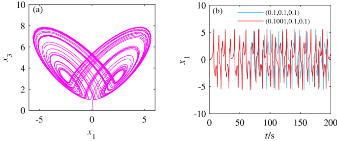
unknown parameter _a_ is assigned a value of \(a = 3\) and the initial value is selected as (0.1,0.1,0.1). The chaotic attractor diagram of system (2) is shown in Fig. 1a. Meanwhile, to

study the sensitivity of system (2) to the initial value, we compare the sequence diagrams with the initial value (0.1001,0.1,0.1) and with the initial value (0.1,0.1,0.1). Figure 1b shows

the effect of small changes in initial values on the dynamic behavior of system (2). The chaotic characteristics of system (2) have obviously changed, indicating that system (2) is

susceptible to the initial value. EQUILIBRIUM POINTS OF THE NEW SYSTEM The left end of the equation for system (2) is assigned to: $$\begin{aligned} \left\{ \begin{array}{lll}

0=-ax_1+x_2x_3\\ 0=ax_1-x_1x_3\\ 0=-ax_3+x_1^2+a\\ \end{array} \right. \end{aligned}$$ (3) The equilibrium points of the system: \(E_1=(0,0,1)\), \(E_2=(-\sqrt{a(a-1)},-\sqrt{a(a-1)},a)\),

and \(E_3=(\sqrt{a(a-1)},\sqrt{a(a-1)},a)\). Because system (2) has chaotic attractor when parameter \(a = 3\), the selected parameter value is substituted at the equilibrium point \(E_1=(0,

0, 1)\), the Jacobian matrix _J_ of the system can be obtained: $$\begin{aligned} J = \left[ \begin{array}{ccc} -a &{} x_3 &{} x_2 \\ a-x_3 &{} 0 &{} -x_1 \\ 2x_1 &{} 0

&{} -a \end{array} \right] = \left[ \begin{array}{ccc} -3 &{} x_3 &{} x_2 \\ 3-x_3 &{} 0 &{} -x_1 \\ 2x_1 &{} 0 &{} -3 \end{array} \right] \end{aligned}$$ (4) The

eigenvalues of the corresponding Jacobian matrix should satisfy the following equation: $$\begin{aligned} f(\lambda )={\lambda }^3+A_2{\lambda }^2+A_1\lambda +A_0 \end{aligned}$$ (5) where

\(A_2=15x_3-5x_3^2\), \(A_1=15-2x_1x_2+3x_3-x_3^2\), and \(A_0=8\). According to the Routh-Hurwitz criterion, the system has a stable equilibrium point when \(A_0>0,A_2>0,\) and

\(A_2A_1-A_0>0\). The corresponding characteristic roots and the types of equilibrium points are obtained as shown in Table 2. Table 2 shows that the characteristic root obtained by

substituting the equilibrium point \(E_1\) into the characteristic equation contains one positive real root and two negative real roots, indicating that the equilibrium point \(E_1\) is a

saddle-focus equilibrium point with index 143. Substituting the equilibrium points \(E_2\) and \(E_3\) into the characteristic equation, the characteristic root contains a negative real root

and a pair of conjugate complex roots with positive real parts, indicating that the equilibrium points \(E_2\) and \(E_3\) are saddle-focus equilibrium points with index 2. EFFECT OF

VARIABLE PARAMETERS ON THE DYNAMIC BEHAVIOR OF THE NEW SYSTEM We study the dynamic behavior of system (2) under the changes of unknown parameters. The initial value is selected as

(0.1,0.1,0.1). Parameter _a_ is taken as the control parameter, and its Lyapunov exponent and bifurcation diagram are shown in Fig. 2a,b respectivly. The system’s dynamic characteristics are

analyzed in Table 3. When \(a\in [3,15]\), the numerical changes of the Lyapunov exponents \(L_1\), \(L_2\), and \(L_3\) in Fig. 2a indicate that the dynamic behavior of system (2) is

complex, and there are periodic, double-period, and chaotic transitions. Figure 2 and Table 2 show that system (2) is in a chaotic state when \(a\in [3,3.78]\), \(a\in [5.12,6.12]\), \(a\in

[8.7,11]\) and \(a\in [13.6,15]\); in a periodic state when \(a\in [3.78,5.12]\); and in a period-doubling state when \(a\in [6.12,8.7]\), and \(a\in [11,13.6]\). Figure 3 depicts the

attractor diagrams of the special value point of parameter _a_. The value of parameter _a_ increases from 3, and there is an internal crisis bifurcation in \(a\cong {3.78}\), \(a\cong

{8.7}\) and \(a\cong {13.6}\). The chaotic attractor collides with the unstable periodic orbit in the attractor basin, causing the attractor to increase. Comparing the Lyapunov exponent

diagram, the attractor is in a period-doubling state at the critical point of period and chaos. At \(a\cong {7.1}\), the system appears jump bifurcation, and there is a phenomenon of

transition from period doubling to period doubling. When the value of parameter _a_ begins to decrease from 15, there is a tangent bifurcation phenomenon in \(a\cong {11}\) and \(a\cong

{6.12}\). At this time, the stable nodes and saddle points of the system are combined or separated to produce orbits with chaotic periods and fixed oscillation periods44. By comparing Fig. 3

with Fig. 2, system (2) has the mutual conversion among periodic state, period doubling state and chaotic state when the values of unknown parameters are different, and the trajectories are

quite different. THE EFFECT OF THE NUMBER OF UNKNOWN PARAMETERS ON THE SYSTEM DYNAMIC BEHAVIOR System (2) contains four unknown parameters with consistent value changes. The change of the

value of unknown parameters will cause the dynamic behavior of the chaotic system to change. Many existing articles literatures45,46 study the dynamic behavior of chaotic systems, the change

of the system’s dynamic behavior is usually explored by varying the parameter value range of the system. Since the unknown parameters of the chaotic system constructed in this paper vary in

the same range, this study changes the number of unknown parameters in system (2) to explore the effect of unknown parameters on the dynamic behavior of system (2). According to Fig. 3a,

system (2) has a chaotic attractor when \(a = 3\); therefore, the unknown parameter _a_ is assigned \(a = 3\). Based on the assigned value of _a_ in system (2), the chaotic system with an

adjustable number of unknown parameters can be obtained. Now a chaotic system with only one unknown parameter, given by system (6), is selected and compared with a chaotic system with two

identical unknown parameters, given by system (7). This demonstrates the effect of unknown parameters on the dynamical behavior of chaotic systems. The obtained chaotic system with only one

unknown parameter is shown in system (6); a chaotic system with two identical unknown parameters is shown in system (7). $$\begin{aligned}{} & {} \left\{ \begin{array}{lll}

\dot{x_1}=-ax_1+x_2x_3\\ \dot{x_2}=3x_1-x_1x_3\\ \dot{x_3}=-3x_3+x_1^2+3\\ \end{array} \right. \end{aligned}$$ (6) $$\begin{aligned}{} & {} \left\{ \begin{array}{lll}

\dot{x_1}=-ax_1+x_2x_3\\ \dot{x_2}=ax_1-x_1x_3\\ \dot{x_3}=-3x_3+x_1^2+3\\ \end{array} \right. \end{aligned}$$ (7) According to Fig. 2, the value range of the unknown parameter _a_ is

selected as \(a\in [2, 6]\). The bifurcation diagram of Fig. 4 shows the difference between the dynamic behavior of systems (6) and (7), indicating the sensitivity of the chaotic system to

the initial conditions. Figure 4a and b clearly show that the dynamic behavior of the chaotic system (2) has changed significantly after varying the number of the same unknown parameters. To

fully illustrate the actual existence of this difference, SE complexity and C0 complexity47 are selected to further prove this phenomenon. The complexity measurement provides a certain

analysis basis for studying the system’s dynamic behavior. Considering the unknown conditions of parameter \(a\in [2,6]\), and initial value (0.1,0.1,0.1), the comparative analysis of

systems (6) and (7) complexity is shown in Fig. 5. From Fig. 4 and Fig. 5, under the premise of determining the value range of unknown parameters for systems (6) and (7), the variation

trends of SE complexity and C0 complexity are consistent with the change in the concentration point of the bifurcation diagram. It is further shown that the dynamic behavior of system (2)

changes when the number of unknown parameters varies. EXPONENTIAL VARIATION CHARACTERISTICS OF NONLINEAR TERMS OF THE NEW SYSTEM DYNAMICS CHANGE CAUSED BY EXPONENTIAL CHANGE By analyzing the

dynamic behavior of system (2), the power index of a single variable in the nonlinear term of system (2) is variable. To explore the effect of the power index change of a single variable in

the nonlinear term of system (2) on the chaotic system, this paper will illustrate this phenomenon by examples. By adding state variables to system (2), a new system (8) is obtained as

follows: $$\begin{aligned} {\left\{ \begin{array}{lll} \dot{x_1}=-ax_1+x_2F_m^i\\ \dot{x_2}=ax_1-x_1F_m^k\\ \dot{x_3}=-ax_3+x_1^2+a\\ \end{array} \right. } \end{aligned}$$ (8) In (8),

\(F_m^i=x_3^i\), \(F_m^k=x_3^k\) and \(i,k\in [1,+\infty )\). \(F_m^i\) and \(F_m^k\) are state variables. The _i_ and _k_ have the following situations: $$\begin{aligned} {\left\{

\begin{array}{lll} i_{(1)}=k_{(1)}+1,\\ i_{(2)}=k_{(2)}-1,\\ i_{(3)}=k_{(3)}\\ \end{array} \right. } \end{aligned}$$ (9) To explore the effect of \(F_m^i\) and \(F_m^k\) on the chaotic

attractor in system (8), the dissipation degree \(\nabla {V}\) of system (8) is calculated: $$\begin{aligned} \nabla {V}=\frac{\partial {\dot{x_1}}}{\partial {x_1}}+\frac{\partial

{\dot{x_2}}}{\partial {x_2}}+\frac{\partial {\dot{x_3}}}{\partial {x_3}}=-a+0-a=-2a \end{aligned}$$ (10) The value of _a_ is positive, indicating that system (8) will eventually form a

dissipation \(\nabla {V}\) of the chaotic attractor over time, and that the formation of the chaotic attractor of system (8) is not affected by \(F_m^i\) and \(F_m^k\). Now select the

appropriate values of _i_ and _k_ to further explore the dynamic behavior of the chaotic system. Select \(i_{(3)}=k_{(3)}=2,3\) respectively to obtain systems (11) and (12):

$$\begin{aligned}{} & {} \left\{ \begin{array}{lll} {\dot{x}}_{1}=-ax_1+x_2x_3^2\\ {\dot{x}}_{2}=ax_1-x_1x_3^2\\ {\dot{x}}_{3}=-ax_3+x_1^2+a\\ \end{array} \right. \end{aligned}$$ (11)

$$\begin{aligned}{} & {} \left\{ \begin{array}{lll} {\dot{x}}_{1}=-ax_1+x_2x_3^3\\ {\dot{x}}_{2}=ax_1-x_1x_3^3\\ {\dot{x}}_{3}=-ax_3+x_1^2+a\\ \end{array} \right. \end{aligned}$$ (12)

The initial value is selected as (0.1, 0.1, 0.1), and the range of unknown parameter _a_ is \(a\in [3,10]\). The bifurcation diagrams of systems (11) and (12) are obtained, as shown in Fig.

6. Figure 6 shows that when \(i_{(3)} = k_{(3)} = 2\), the dynamic behavior of system (8) shows the alternation of the period, period doubling and chaos; further, the frequency of

alternation varies with the value of _i_ and _k_. Simultaneous increases in the value of _i_ and _k_ result in an increase in the highest power of the system’s nonlinear terms. This changes

the chaotic properties of the system as well as the trajectory of the chaotic attractors present in the system. When \(i_{(3)} = k_{(3)}\), the value of \(i_{(3)}\) and \(k_{(3)}\) tend to

be infinite, the highest power of the nonlinear terms in system (8) is positive infinity, and the system has chaotic characteristics. To clearly show the dynamic characteristics of system

(8) when the value of _i_ and _k_ change, the Poincare sections of \(x_1\) and \(x_2\) planes are selected with \(a = 4.5\), \(i_{(3)}\) = \(k_{(3)}\) = 2,3,4, and 6, and \(x_3=2\), as shown

in Fig. 7. Select the quantitative relationships between _i_ and _k_ as \(i_{(1)} = k_{(1)} + 1\) and \(i_{(2)}\)= \(k_{(2)}-1\). The initial value of system (8) is (0.1, 0.1, 0.1), the

unknown parameter value ranges are \(a \in { [2, 6]}\). When \(i_{(1)}\)= \(i_{(2)}\)= 2 and \(i_{(1)}\) = \(i_{(2)}\) = 4 are selected respectively, the bifurcation diagrams of system (8)

under two different values are shown in Fig. 8. Figure 8 shows that in two different states of \(i= k\), the chaotic characteristics of system (8) are very different by comparing the

presence of dense points in the bifurcation diagram at different times. When the quantitative relationship between _i_ and _k_ is \(i_{(3)}\ne {k_{(3)}}\), the speed of dynamic behavior

transformation of \(i>{k}\) is faster than that of \(i<k\) in the same time. According to Figs. 7 and 8, as the values of _i_ and _k_ increase, the motion trajectory of the chaotic

attractor of system (8) changes; this shows that under certain value conditions, the change of _i_ and _k_ values will affect the dynamic behavior of the system. 0–1 TEST To further show the

dynamic behavior of the system with different \(i_{(m)}\) and \(k_{(n)}\) values, this paper uses the 0–1 test method to explore the new system. Here, by comparing the dynamic behavior of

the system when the same unknown parameters are taken in systems (11) and (12), we further illustrate the effect of the exponential value change on the dynamic behavior of the system. The

improved 0–1 test algorithm48,49 used in this paper defines the following equation: $$\begin{aligned} \left\{ \begin{array}{lll} p(n)=\sum \limits ^{n}_{j=1}\phi (j){\textrm{cos}}(\theta

(j)),n=1,2,3\cdots \\ s(n)=\sum \limits ^{n}_{j=1}\phi (j){\textrm{sin}}(\theta (j)),n=1,2,3\cdots \\ \end{array} \right. \end{aligned}$$ (13) In (13), \(\phi (j)\) represents an observable

dataset and \(\theta (j)=jc+\sum \limits _{i=1}^{j}\phi (i)\), \(j=1,2,3,\cdots ,n\). On the basis of _p_(_n_), the root mean square displacement is defined: $$\begin{aligned} M(n)=\mathop

{\textrm{lim}}\limits _{N\rightarrow \infty }\frac{1}{N}\sum \limits ^{n}_{j=1}[p(j+n)-p(j)]^2,n=1,2,3,\cdots \end{aligned}$$ (14) When the behavior of _p_(_n_) or _s_(_n_) is in Brownian

motion, the RMS displacement _m_(_n_) increases linearly with time. When the behavior of _p_(_n_) or _s_(_n_) is bounded, then the RMS displacement _M_(_n_) is also bounded. For systems (13)

and (14), 0–1 test is conducted when the values of unknown parameter _a_ are set as \(a=3\) and \(a=6.25\). The resulting state space diagrams are shown in Fig. 9. Figure 9 depicts the

apparent difference between the state space diagram of systems (13) and (14), which corresponds to the dynamic behavior in the bifurcation diagram of Fig. 6. It further indicates that the

numerical value of the exponential of the nonlinear term in system (10) change the system’s dynamic behavior. CIRCUIT SIMULATION ANALYSIS To verify the feasibility of circuit implementation

of system (8), the circuit diagram of system (8) is set up when the value range of index \(i_{(m)}\) and \(k_{(n)}\) are positive natural number as shown in Fig. 10. The operational

amplifier (LM324M) and other related components are used for related operations such as addition, subtraction and integration. Apply Kirchhoff’s law to Fig. 10 to get the differential

equation: $$\begin{aligned} {\left\{ \begin{array}{lll} \dot{x}_1=-\frac{1}{C_1R_{13}}x_1+\frac{R_7}{C_1R_3R_4}x_2x_3^{i}\\ \\ \dot{x}_2=\frac{R_1}{C_2R_2R_5}x_1-\frac{1}{C_2R_6}x_1x_3^{k}\\

\\ \dot{x}_3=-\frac{1}{C_3R_{12}}x_3+\frac{R_8}{C_3R_9R_{10}}{U_1}+\frac{R_1}{C_3R_2R_{11}}x_1^2\\ \end{array} \right. } \end{aligned}$$ (15) The capacitors are set to

\(C_1=C_2=C_3=1\textrm{uF}\), and the other corresponding resistance values of system (15) are as follows: $$\begin{aligned} \left\{ \begin{array}{lll} R_3=R_6=R_{11}=1000{\textrm{k}{\Omega

}}\\ R_1=R_2=R_4=R_7=10{\textrm{k}{\Omega }}\\ R_8=1{\textrm{k}{\Omega }},R_9=10{\textrm{k}{\Omega }},R_{10}=100{\textrm{k}{\Omega }}\\ \end{array} \right. \end{aligned}$$ (16) Among them,

the values of \(R_5\), \(R_{12}\), \(R_{13}\) and the voltage \(U_1\) can be adjusted to match the value of the unknown parameter _a_ in system (8). When the unknown parameter is \(a=3\),

select \(R_5= R_{12}= R_{13}=333.33\textrm{k}{\Omega }\), \(U_1=3\textrm{V}\), a multiplier (AD633) with an output gain of 1, and the exponent of the state variable \(x_3\) of the nonlinear

term in system (8) as a variable parameter. The circuit simulation diagrams of parameters _i_ and _k_ with different values are obtained, as shown in Fig. 11. Figure 11 shows that the

simulation effect matches the dynamic behavior of the corresponding period. The dynamic behavior of system (8) under different initial conditions is further verified, which provides a

theoretical reference for the hardware implementation of system (8). IMAGE ENCRYPTION PROCESSING To explore the relative performance of encryption and decryption exhibited by the chaotic

system with the same unknown parameters applied to the image encryption system, this paper applies system (2) to the chaotic image encryption system with the same encryption and decryption

process. The image encryption system with the same encryption process and decryption process adopted in this paper mainly includes five parts: cipher generation, forward diffusion,

correlation scrambling, image rotation and backward diffusion. Among them, the encryption system uses a scrambling algorithm associated with plaintext. A schematic diagram of the structure

of the image cryptography system based on system (2) is shown in Fig. 12. Given that the plaintext image _P_ size is \(M\times {N}\), the gray level is _L_ bits, and \(\textrm{mod} (N,2)=0\)

is satisfied. When \(\textrm{mod} (N,2)\ne 0\), it is necessary to add a column vector of all 0s to the \(M\times {1}\) column of image _P_ to obtain a new image of size \(M\times (N+1)\).

The selected key is \(K=[x_0,y_0,z_0,r_1,r_2]\), where \(x_0,y_0,z_0\) are the initial value of system (2), and \(r_1\) and \(r_2\) are the 8-bit random number. The password generation

module application generates 6 pseudo-random matrices, denoted as _X_, _Y_, _Z_, _V_, _U_, and _W_ with size of \(M\times {N}\). * STEP 1: Select \(x_0,y_0,z_0\) in the key _K_ as the

initial value of system (2), and iterate system (2) \(r_1+r_2+MN\) times to obtain 3 pseudo-random sequences \(x_i\), \(y_i\), \(z_i\), \(i=1,2,3\cdots {MN}\) * STEP 2: Apply the following

equation to the pseudo-random sequence. \({x_i}\), \(y_i\), \({z_i}\) and generate the matrix _X_, _Y_, _Z_, _G_, _U_,  and _Q_. $$\begin{aligned} \left\{ \begin{array}{lll}

X(u,v)={\mathrm{mod(floor}}(x_{(u-1)\times {N}}\times {10^{15}}),2^L)\\ Y(u,v)={\mathrm{mod(floor}}(y_{(u-1)\times {N}}\times {10^{14}}),2^L)\\ Z(u,v)={\mathrm{mod(floor}}(z_{(u-1)\times

{N}}\times {10^{13}}),N)+1\\ G(u,v)={\mathrm{mod(floor}}(x_{(u-1)\times {N}}+z_{(u-1)\times {N}}\times {10^{12}}),M)+1\\ U(u,v)={\mathrm{mod(floor}}(y_{(u-1)\times {N}}+z_{(u-1)\times

{N}}\times {10^{11}}),M)+1\\ Q(u,v)={\mathrm{mod(floor}}(y_{(u-1)\times {N}}+y_{(u-1)\times {N}}\times {10^{10}}),M)+1\\ \end{array} \right. \end{aligned}$$ (17) * STEP 3: Use the

pseudo-random matrix _X_ and \(r_1\) to perform forward diffusion processing on the plaintext image _P_, and apply the exclusive OR operation to obtain the matrix _A_: $$\begin{aligned}

\left\{ \begin{array}{lll} A(1,1)=P(1,1)\oplus {X(1,1)}\oplus {r_1}\\ A(1,j)=P(i,1)\oplus {X(i,1)}\oplus {E(1,j-1)}\\ A(i,1)=P(i,1)\oplus {X(i,1)}\oplus {E(i-1,N)}\oplus {E(i-1,1)}\\

A(i,j)=P(i,j)\oplus {X(i,j)}\oplus {E(i-1,j)}\oplus {E(i,j-1)}\\ \end{array} \right. \end{aligned}$$ (18) In (18), \(i=2,\cdots ,\) \(M,j=2,\cdots ,N\). * STEP 4: Rotate the matrix _A_

\(180^0\) to obtain the matrix \(\theta \). * STEP 5: Using pseudo-random matrices _Z_, _G_, _U_ and _Q_ to scramble the explicit association of matrix \(\theta \), the method is as follows:

Replace the pixel position \(\theta =(i, j)\) with \(\theta =({\overline{k}},{\overline{s}})\). If mod(_N_,2)=0, then \({\overline{k}}\) and \({\overline{s}}\) are calculated according to

system (19). $$\begin{aligned} \left\{ \begin{array}{lll} \bar{k}=(M+1)-({\textrm{mod}}(U(i,j))+{\textrm{sum}}(\theta (G(i,j),1:N)),M)+1)\\

\bar{s}=(N+1)-({\textrm{mod}}(Q(i,j))+{\textrm{sum}}(\theta (1:M,Z(i,j))),N)+1)\\ \end{array} \right. \end{aligned}$$ (19) If mod\((N,2)\ne {0}\), then use the following system (20) to

calculate \(\bar{k},\bar{s}\). $$\begin{aligned} \left\{ \begin{array}{lll} \bar{k}={\textrm{mod}}(U(i,j)+{\textrm{sum}}(\theta {(G(i,j),1:N)}),M)+1\\

\bar{s}={\textrm{mod}}(Q(i,j)+{\textrm{sum}}(\theta {(1:M,Z(i,j))}),N)+1\\ \end{array} \right. \end{aligned}$$ (20) STEP 6: When \(\bar{k}=i\), or \(\bar{s}=j\), or \({\bar{k}}= V(i,j)\), or

\(\bar{s}=Z(i,j)\), or \(G(i,j)=i\), or \(Z(i,j)=j\), keep the position of \(\theta (i,j)\) unchanged, otherwise replace \(\theta =(i, j)\) with \(\theta =(\bar{k},\bar{s})\). * STEP 7:

According to the order from left to right and top to bottom, process the position of each pixel of matrix \(\theta \), and repeat STEP 5 and STEP 6. The scrambling algorithm used in the

encryption and decryption processes is the same, but the cipher matrix is different. The cipher matrix corresponding to the decryption process is as follows: $$\begin{aligned} \left\{

\begin{array}{lll} &{}\widetilde{X}={\textrm{rot}}180(X),\widetilde{Y}={\textrm{rot}}180(Y),\widetilde{Z}=(N+1)-{\textrm{rot}}180(Z)\\

&{}\widetilde{Q}={\textrm{rot}}180(W),\widetilde{U}={\textrm{rot}}180(U),\widetilde{G}=(M+1)-{\textrm{rot}}180(V)\\ \end{array} \right. \end{aligned}$$ (21) * STEP 8: Perform \(180^0\)

rotation processing on the scrambled matrix \(\theta \) to obtain the matrix _F_. * STEP 9: Use pseudo-random matrices _Y_ and \(r_2\) to perform backward diffusion processing on the

plaintext image _F_, and apply the exclusive OR operation to obtain the matrix _H_: $$\begin{aligned} \left\{ \begin{array}{lll} H(M,N)=F(M,N)\oplus {Y(M,N)}\oplus {r_2}\\

H(M,j)=F(M,j)\oplus {Y(M,j)}\oplus {F(M,j+1)}\\ H(i,N)=F(i,N)\oplus {Y(i,N)}\oplus {F(i+1,1)\oplus {F(i+1,N)}}\\ H(i,j)=F(i,j)\oplus {Y(i,j)}\oplus {F(i+1,j)\oplus {F(i,j+1)}}\\ \end{array}

\right. \end{aligned}$$ (22) In (22), \(i=M-1,\cdots ,1,\) \(j=N-1,\cdots ,1\). * STEP 10: Rotate the matrix _H_ \(180^0\) to obtain the matrix _B_, which is the ciphertext image. . The

encryption process is summarized in Fig. 13. The encryption process of the algorithm is the same as the decryption process. At the same time, unlike the classical image cryptosystem, the

algorithm does not have a loop operation, only contains two diffusion and a scrambling operation. Since only the scrambling algorithm associated with the plaintext is used, the diffusion

algorithm has nothing to do with the plaintext. Thus the confidentiality effect is stronger. SIMULATION RESULTS AND PERFORMANCE ANALYSIS ENCRYPTION AND DECRYPTION OF IMAGES This section

mainly analyzes the relevant encryption and decryption performance of the grayscale diagram of this chaotic encryption system. All of the following simulation experiments are implemented on

Matlab2017b and the computer’s associated configuration of 12GB RAM and Intel(R)Core(TM) i5-7200U CPU @ 2.50GHz 2. The simulation used a grayscale map of Brick Wall, Sand, Motion, Grass, and

Toy Vehicle, with all five images having 512 \(\times \) 512 pixels. The key \(K=[x_0,y_0,z_0,r_1,r_2]\) is selected, where \(x_0,y_0,\) and \(z_0\) are the initial values of system (2),

and \(r_1\) and \(r_2\) are the 8-bit random number (\(r_1,r_2\in [0,255]\)). The unknown parameter _a_ of system (2) is assigned of \(a=3\). The key is selected as \(x_0,y_0,z_0\in

[-50,50]\), and the step length is selected as 1/_t_, where \(t=10^{14}\). The size of the key space is 6.5536\(\times {10^{52}}\). The key is selected as \(K=[ -40.1, 40.1, -35.7, 100.0,

235.0]\) to obtain plaintext, encrypted and decrypted images based on system (2), as shown in Fig. 14. Figure 14 shows that the encryption and decryption effect of the encryption system is

remarkable. In the figure, the histogram of the ciphertext rendering is evenly distributed, which can effectively resist the attack and obtain useful information. ENCRYPTION AND DECRYPTION

TIME TEST The image encryption system is ultimately applied to actual life, and there are specific requirements for the encryption and decryption time. The encryption and decryption time of

the image encryption system must be efficient and fast. The article tests the encryption and decryption time of different pixel grayscale maps twenty times and chooses the average. The

resulting test results are shown in Table 4. The time of encryption and decryption of the grayscale map under different pixels shown in Table 4 can better show the superiority of the

encryption system in the encryption and decryption time and has a great possibility of being applied to the production practice. NIST TEST Chaotic pseudo-random sequences are an important

part of the chaotic image cryptography system, and the password of the image encryption system has excellent statistical characteristics. Typically, chaotic sequences used for image

encryption must pass the pseudo-random sequence test. NIST50,51 is a typical test method, and the test results are authoritative. The chaotic sequence used for the image encryption system

has strong statistical characteristics; this is the basis for the perfect success of the image encryption system, NIST test for the chaotic sequences is selected for this article. Table 5

shows the test results. Table 5 shows that the chaotic sequence successfully passed 15 test experiments, which proves that the chaotic sequence used in the image encryption system in this

paper has excellent statistical characteristics. \(\CHI ^2\) TEST Figure 14 shows that there are obvious differences between the histogram of the plaintext image and the histogram of the

ciphertext image. The histogram image of the plaintext image is irregular, and the histogram of the encrypted image is relatively flat. To further explore the quantitative difference between

the histogram of a plaintext image and the histogram of a redaction image, the \(\chi ^2\) statistic (unilateral hypothesis detection) is used to measure the quantitative difference between

them. Using the Pearson \(\chi ^2\) statistic Eq. (23) follows a \(\chi ^2\) distribution with \(n-1\) degrees of freedom. Image size is \(M\times {N}\), assuming that grayscale pixels

\(f_i\) in the histogram follow an even distribution with \(i=0,1,2,\cdots ,255\). $$\begin{aligned} \chi ^2=\sum ^{255}_{i=0}\frac{(f_i-g)^2}{g},\ \ g=(M\times {N})/256 \end{aligned}$$ (23)

The significance levels \(\alpha =0.05\) and \(\chi ^2_{0.05}=284.33591\) are selected. The \(\chi ^2\) test results for plaintext images and ciphertext images of Brick Wall, Sand, Motion,

Grass, and Toy Vehicle are shown in Table 6. The calculated values of the \(\chi ^2\) statistic of the five plaintext images in Table 6 are significantly greater than that of \(\chi

^2_{0.05}(255)\), and the calculated values of the \(\chi ^2\) statistic of the ciphertext images are significantly less than that of \(\chi ^2_{0.05}(255)\); this can be considered to be

approximately evenly distributed in the histogram of the ciphertext image in Fig. 14, indicating that the encryption algorithm can resist the attack well. INFORMATION ENTROPY ANALYSIS

Information entropy reflects the uncertainty of image information to a certain extent. In general, the larger the value of information entropy, the less visual information. The equation for

calculating the expression of information entropy is: $$\begin{aligned} H=-\sum ^L_{i=0}p(i){\textrm{log}}_2p(i) \end{aligned}$$ (24) where _L_ is the number of gray levels of the image and

_p_(_i_) is the probability of gray value _i_ appearing. The images are selected as 8 bits, and the outstanding value of information entropy is 8. The entropy of information in plaintext and

ciphertext is calculated, and the table of changes in information entropy is shown in the Table 7. Table 7 shows the values of the entropy of plaintext images and ciphertext images. The

information entropy value of the plaintext is quite different from the theoretical value, and the information entropy value of the ciphertext is close to the ideal information entropy value,

indicating that the encryption system has a better encryption effect on system (2). KEY SENSITIVITY ANALYSIS Key sensitivity is mainly used to analyze the difference between two ciphertext

images obtained by encrypting the same plaintext image when the key changes in the image encryption system. Since a good image encryption system has strong key sensitivity, it is

particularly important to test the key sensitivity of the image encryption system. In this section, we select the initial value of system (2) as \(K = [x_0, y_0, z_0, r_1, r_2]\), where

\(x_0, y_0, z_0\in [50, 50]\), \(r_1\) and \(r_2 \in [0, 255]\), at steps of \(10^{-14}\). As a test for _K_, 1000 values are randomly selected from the keyspace. For each set of keys to

vary a specific number of the variable, each change is in a step of \(10^{-14}\). Further, the same plaintext image is encrypted with the key before and after the change in order to compare

the two ciphertext images obtained. NPCR and UACI52 must investigate the performance indicators for image encryption, which is defined as: assuming that two plaintext images \(P_1\) and

\(P_2\) are the same except for the value difference of 1 at a pixel (_q_, _p_), the same chaotic encryption system is used to encrypt the plaintext image to obtain the corresponding

ciphertext images \(C_1\) and \(C_2\): $$\begin{aligned}{} & {} G(q,p) = \left\{ \begin{array}{lll} 0,\quad C_1(q,p)=C_2(q,p)\\ 1,\quad C_1(q,p)\ne C_2(q,p)\\ \end{array} \right.

\end{aligned}$$ (25) $$\begin{aligned}{} & {} \left\{ \begin{array}{lll} {\textrm{NPCR}}=\frac{1}{M\times {N}}\sum \limits ^M_{q=1}\sum \limits ^N_{p=1}{G(q,p)}\times 100\%\\

{\textrm{UACI}}=\frac{1}{M\times {N}}\sum \limits ^M_{q=1}\sum \limits ^N_{p=1}\frac{\vert C_1(q,p)-C_2(q,p)\vert }{255-0}\times 100\%\\ \end{array} \right. \end{aligned}$$ (26) According to

the calculated value given in Ref.53, the theoretical value of NPCR is 99.5893% when the plaintext image is \(512\times 512\), and the theoretical value interval of UACI is (33.3730%,

33.5541%). Use the Brick Wall, Sand, Motion, Grass and Toy Vehicle image to test. The calculated values for NPCR and UACI are shown in Table 8. The test results of NPCR and UACI in Table 8

all meet the theoretical numerical requirements, indicating that all passed the test. To further explore the sensitivity of the key in the encryption and decryption process, we select a set

of \(K_a=[-35.5,-15.4,25.6,111,222]\) in the key space, and add an increment to it to obtain \(K_b=[-35.5+10^{-14},-15.4,25.6,111,222]\) as the wrong key. Use the Brick Wall image to test,

and the test results are shown in Fig. 15. Through the key sensitivity test, Fig. 15 shows that when there is a small error in the value of the key space, the decryption result will be

biased, resulting in a mismatch between the decrypted image and the plaintext image. The key space is strongly sensitive to the value of the key. NOISE ATTACK DETECTION To further explore

the anti-interference performance of the chaotic encryption system proposed in this paper, the noise intensity of 0.05 and 0.1 is added to the encryption and decryption test, and the

obtained anti-interference effect diagram is shown in Fig. 16. Figure 16 shows the decrypted image obtained by decoding the encrypted image with different intensities of salt and pepper

noise has excellent discrimination. The encryption algorithm is robust to noise attacks and has excellent security performance. CLEAR TEXT SENSITIVITY ANALYSIS With the help of the same key,

the plaintext sensitivity test uses an image encryption system to encrypt two slightly different plaintext images. The corresponding ciphertext image is obtained, and the sensitivity of the

image encryption system to the plaintext is reflected by comparing the differences in the obtained ciphertext images. To test the sensitivity of the image encryption system used in this

article to clear text, the classic plaintext image is selected as the experimental test image. Select \(K_a=[-35.5,-15.4,25.6,111,222]\), which compares the values of NPCR and UACI of two

plaintext images by varying the value of a pixel in the plaintext image and encrypting it again. Through repeated calculations, the plaintext sensitivity analysis results of the chaotic

encryption system are shown in Table 9. After analyzing the clear text sensitivity results of the chaotic encryption system in Table 9, the calculation results of NPCR and UACI are similar

to the theoretical values after the plaintext images with minor pixel differences are encrypted. The results illustrates that the chaotic image encryption system proposed in this paper has

prominent plaintext sensitivity. CORRELATION ANALYSIS OF ENCRYPTION SYSTEM To show the correlation between adjacent pixels after the encryption system processes the plaintext, we randomly

select \(\beta \) pairs of adjacent pixels from the used image. The gray value is \((\mu _i,\lambda _i)\), \(i=1,2,3,\cdots ,\beta \), and then obtain the correlation coefficient _T_.

$$\begin{aligned}{} & {} T=\frac{{\textrm{cov}}(\mu ,\lambda )}{\sqrt{D(\mu )}\sqrt{D(\lambda )}} \end{aligned}$$ (27) $$\begin{aligned}{} & {} {\textrm{cov}}(\mu ,\lambda )=\beta

^{-1}\sum ^{\beta }_{i=1}(\mu _i-E(\mu ))(\lambda _i-E(\lambda )) \end{aligned}$$ (28) $$\begin{aligned}{} & {} D(\rho )=\beta ^{-1}\sum ^\beta _{i=1}(\rho _i-E(\rho ))^2 \end{aligned}$$

(29) $$\begin{aligned}{} & {} E(\rho )=\beta ^{-1}\sum ^\beta _{i=1}\rho _i \end{aligned}$$ (30) Figure 17 shows the correlation between plaintext and ciphertext in various directions.

8000 pairs of adjacent pixels are selected from the horizontal, diagonal and vertical directions, and the correlation coefficients are shown in Table 10. Tables 10 and 11 show the

correlation in each direction of the plaintext that the correlation coefficient value of the plaintext is greater than 0.9, and the pixel-intensive points in the image are all near the

diagonal; this proves that the correlation between adjacent pixels of the chosen plaintext image is powerful. After the encryption system is processed, the correlation coefficient values of

the ciphertext image in all directions are close to 0. The pixel dense points in the image show irregular scattered distribution, indicating that the correlation of ciphertext image is weak;

this proves that the system has good encryption performance. Table 11 compares the correlation of adjacent pixels of Brick Wall image in different directions with the performance of classic

images in other literatures, and observes that the correlation of adjacent pixels in different directions of ciphertext images is close to 0, which further shows that the chaotic encryption

system proposed in this paper has positive encryption and decryption effects. CONCLUSION This study proposes a new improved chaotic system and successfully analyzes the effect of varying

the number of unknown parameters in the new system. The dynamic behavior change of a chaotic system caused by the exponential change of a single-state variable in the nonlinear term of the

new system is compared and analyzed. The results indicate that when the index value range is close to positive infinity, the chaotic system may possibly have a chaotic attractor. Simulation

analysis of the new system under different initial conditions are conducted through circuit simulation. Finally, the new system is successfully applied to an image encryption system, and an

excellent encryption effect is achieved. DATA AVAILABILITY The data that support the findings of this study are available within the article. Further requests can be made to the

corresponding author. REFERENCES * Li, R. G. & Wu, H. N. Secure communication on fractional-order chaotic systems via adaptive sliding mode control with teaching-learning-feedback-based

optimization. _Nonlinear Dynam._ 95(2), 1221–1243 (2019). Article  MATH  Google Scholar  * El-Maksoud, A., El-Kader, A., Hassan, B. G., Rihan, N. G. & Abu-Elyazeed, M. F. FPGA

implementation of sound encryption system based on fractional-order chaotic systems. _Microelectron. J._ 90, 323–335 (2019). Article  Google Scholar  * Tian, A. H., Fu, C. B., Xiong, H. G.

& Yau, H. T. Innovative intelligent methodology for the classification of soil salinization degree using a fractional-order master–slave chaotic system. _Int. J. Bifurcat Chaos._ 29(2),

1950026 (2019). Article  MathSciNet  MATH  Google Scholar  * Niu, Y. J., Sun, X. M., Zhang, C. & Liu, H. Anticontrol of a fractional-order chaotic system and its application in color

image encryption. _Math. Probl. Eng._ 2020, 6795964 (2020). Article  MathSciNet  Google Scholar  * Yu, F., Shen, H., Zhang, Z. N., Huang, Y. Y. & Cai, S. A new multi-scroll Chua’s

circuit with composite hyperbolic tangent-cubic nonlinearity: Complex dynamics, Hardware implementation and Image encryption application. _Integration_ 81, 71–83 (2021). Article  Google

Scholar  * Yu, J. Y., Li, C., Song, X. M. & Wang, E. F. Parallel mixed image encryption and extraction algorithm based on compressed sensing. _Entropy-Switz._ 23(3), 278 (2021). Article

  ADS  Google Scholar  * Martines-Arano, H., Vidales-Hurtado, M. A., Palacios-Barreto, S., Valdez, M. T. & Torres, C. T. Sequential photodamage driven by chaotic systems in NiO thin

films and fluorescent human cells. _Processes_ 8(11), 1377 (2020). Article  CAS  Google Scholar  * Vijayakumar, B., Rajendar, G. & Ramaiah, V. Optimal location and capacity of Unified

Power Flow Controller based on chaotic krill herd blended runner root algorithm for dynamic stability improvement in power system. _Int. J. Numer. Model. El._ 34(2), 1–28 (2020). Google

Scholar  * Eema, B. & Kma, C. Control and synchronization of the hyperchaotic attractor for a 5-D self-exciting homopolar disc dynamo. _Alex. Eng. J._ 60(1), 1173–1181 (2021). Article 

Google Scholar  * Lai, Q., Wan, Z., Kuate, P. & Fotsin, H. Coexisting attractors, circuit implementation and synchronization control of a new chaotic system evolved from the simplest

memristor chaotic circuit. _Commun. Nonlinear. Sci._ 89, 105341 (2020). Article  MathSciNet  MATH  Google Scholar  * Yu, F. _et al._ Dynamic analysis, circuit design, and synchronization of

a novel 6D memristive four-wing hyperchaotic system with multiple coexisting attractors. _Complexity_ 2020, 5904607 (2020). MATH  Google Scholar  * Deng, Q. L., Wang, C. H. & Yang, L. M.

Four-wing hidden attractors with one stable equilibrium point. _Int. J. Bifurcat. Chaos._ 30(06), 2050086 (2020). Article  MathSciNet  MATH  Google Scholar  * Yang, J. P. & Liu, Z. R. A

novel simple hyperchaotic system with two coexisting attractors. _Int. J. Bifurcat. Chaos._ 29(14), 1950203 (2019). Article  MathSciNet  MATH  Google Scholar  * Bao, B. C., Hu, F. W., Chen,

M., Xu, Q. & Yu, Y. J. Self-excited and hidden attractors found simultaneously in a modified Chua’s circuit. _Int. J. Bifurcat. Chaos._ 25(5), 1550075 (2015). Article  MATH  Google

Scholar  * Chen, M. _et al._ Dynamics of self-excited attractors and hidden attractors in generalized memristor-based Chua’s circuit. _Nonlinear. Dynam._ 81(1–2), 215–226 (2015). Article 

MathSciNet  MATH  Google Scholar  * Li, C. B. & Sprott, J. C. Coexisting hidden attractors in a 4-D simplified Lorenz system. _Int. J. Bifurcat. Chaos._ 24(3), 1450034 (2014). Article 

MathSciNet  MATH  Google Scholar  * Liu, X. & Ma, L. Chaotic vibration, bifurcation, stabilization and synchronization control for fractional discrete-time systems. _Appl. Math. Comput._

385, 125423 (2020). MathSciNet  MATH  Google Scholar  * Chen, Y. M. Dynamics of a Lorenz-type multistable hyperchaotic system. _Math. Method. Appl. Sci._ 41, 1–12 (2018). Article  ADS 

MathSciNet  Google Scholar  * Ma, C., Mou, J., Xiong, L., Banerjee, S. & Han, X. Dynamical analysis of a new chaotic system: Asymmetric multistability, offset boosting control and

circuit realization. _Nonlinear Dyn._ 103(6), 1–14 (2021). Google Scholar  * Zhou, L., Wang, C. & Zhou, L. Generating four-wing hyperchaotic attractor and two-wing, three-wing, and

four-wing chaotic attractors in 4D memristive system. _Int. J. Bifurcat. Chaos._ 27(02), 1750027 (2017). Article  MathSciNet  MATH  Google Scholar  * Yildirim, M. & Kacar, F. Chaotic

circuit with OTA based memristor on image cryptology. _AEU-Int. J. Electron. C._ 127, 153490 (2020). Article  Google Scholar  * Sahin, M. E., Demirkol, A. S., Guler, H. & Hamamci, S. E.

Design of a hyperchaotic memristive circuit based on Wien bridge oscillator. _Comput. Electr. Eng._ 88(5), 106826 (2020). Article  Google Scholar  * Yan, Y., Ren, K. C., Qian, H. & Yao,

X. Y. Coexistence of periodic and strange attractor in a memristive band pass filter circuit with amplitude control. _Eur. Phys. J. Special. Topics._ 228(10), 2011–2021 (2019). Article  ADS

  Google Scholar  * Jiang, Y. L., Yuan, F. & Li, Y. X. A dual memristive Wien-bridge chaotic system with variable amplitude and frequency. _Chaos_ 30(12), 123117 (2020). Article  ADS 

MathSciNet  PubMed  MATH  Google Scholar  * Liu, T. M., Yan, H. Z., Banerjee, S. & Mou, J. A fractional-order chaotic system with hidden attractor and self-excited attractor and its DSP

implementation. _Chaos. Soliton. Fract._ 145, 110791 (2021). Article  MathSciNet  Google Scholar  * Yan, D. W., Wang, L. D., Duan, S. K., Chen, J. J. & Chen, J. H. Chaotic attractors

generated by a memristor-based chaotic system and Julia fractal. _Chaos Soliton Fract._ 146(7191), 110773 (2021). Article  MathSciNet  Google Scholar  * Sun, J., Li, C., Lu, T., Akgul, A.

& Min, F. A memristive chaotic system with hypermultistability and its application in image encryption. _IEEE Access_ 8, 139289–139298 (2020). Article  Google Scholar  * Zhou, L., You,

Z. & Tang, Y. A new chaotic system with nested coexisting multiple attractors and riddled basins. _Chaos Soliton Fract._ 148, 111057 (2021). Article  MathSciNet  MATH  Google Scholar  *

Alamodi, A., Sun, K. & Peng, Y. Chaotic attractor with varied parameters. _Eur. Phys. J. Spec. Top._ 229(6–7), 1095–1108 (2020). Article  Google Scholar  * Yan, M. X. & Xu, H. A

chaotic system with a nonlinear term and multiple coexistence attractors. _Eur. Phys. J. Plus._ 135(6), 135–452 (2020). Article  ADS  Google Scholar  * Zheng, J. & Hu, H. P. A symmetric

image encryption scheme based on hybrid analog-digital chaotic system and parameter selection mechanism. _Multimed. Tools. Appl._ 80, 20883–20905 (2021). Article  Google Scholar  * X. Wang,

P. Liu, A New Full Chaos Coupled Mapping Lattice and Its Application in Privacy Image Encryption, IEEE. T. Circuits-I., 2021. * Kengne, J., Tsafack, N. & Kengne, L. K. Dynamical analysis

of a novel single Opamp-based autonomous LC oscillator: Antimonotonicity, chaos, and multiple attractors. _Int. J. Dyn. Control_ 6(4), 1543–1557 (2015). Article  MathSciNet  Google Scholar

  * Tsafack, N. _et al._ A memristive RLC oscillator dynamics applied to image encryption. _J. Inf. Secur. Appl._ 61, 102944 (2021). Google Scholar  * Njitacke, Z. T. _et al._ Hamiltonian

energy and coexistence of hidden firing patterns from bidirectional coupling between two different neurons. _Cogn. Neurodyn._ 16(4), 899–916 (2022). Article  PubMed  Google Scholar  *

Nazari, M. & Mehrabian, M. A novel chaotic IWT-LSB blind watermarking approach with flexible capacity for secure transmission of authenticated medical images. _Multimed. Tools. Appls._

80(7), 10615–10655 (2021). Article  Google Scholar  * Soualmi, A., Alti, A. & Laouamer, L. A novel blind medical image watermarking scheme based on Schur triangulation and chaotic

sequence. _Concurr. Comp-Pract. E._ 34(1), e6480 (2022). Article  Google Scholar  * García-Guerrero, E. E., Inzunza-González, E., López-Bonilla, O. R., Cárdenas-Valdez, J. R. &

Tlelo-Cuautle, E. Randomness improvement of chaotic maps for image encryption in a wireless communication scheme using PIC-microcontroller via Zigbee channels. _Chaos. Soliton. Fract._ 133,

109646 (2020). Article  MathSciNet  MATH  Google Scholar  * Trujillo-Toledo, D. A. _et al._ Real-time RGB image encryption for IoT applications using enhanced sequences from chaotic maps.

_Chaos. Soliton. Fract._ 153, 111506 (2021). Article  MathSciNet  Google Scholar  * Sun, K. & Sprott, J. C. Dynamics of a simplified Lorenz system. _Int. J. Bifurcat. Chaos_ 19(04),

1357–1366 (2009). Article  MATH  Google Scholar  * Kingni, S. T. _et al._ Constructing and analyzing of a unique three-dimensional chaotic autonomous system exhibiting three families of

hidden attractors. _Math. Comput. Simulat._ 132, 172–182 (2017). Article  MathSciNet  MATH  Google Scholar  * Nazarimehr, F. _et al._ A new four-dimensional system containing chaotic or

hyper-chaotic attractors with no equilibrium, a line of equilibria and unstable equilibria. _Chaos Soliton Fract._ 111, 108–118 (2018). Article  ADS  MathSciNet  MATH  Google Scholar  *

Cafagna, D. & Grassi, G. New 3D-scroll attractors in hyperchaotic Chua’s circuits forming a ring. _Int. J. Bifurcat. Chaos_ 13(10), 2889–2903 (2003). Article  MathSciNet  MATH  Google

Scholar  * Pomeau, Y. & Manneville, P. Intermittent transition to turbulence in dissipative dynamical systems. _Math. Phys._ 74, 188–197 (1980). Article  ADS  MathSciNet  Google Scholar

  * Guo, M. _et al._ A novel memcapacitor and its application in a chaotic circuit. _Nonlinear Dynam._ 105, 877–886 (2021). Article  Google Scholar  * Og, A., Icc, B. & Jpr, C. Dynamic

behavior in a pair of Lorenz systems interacting via positive-negative coupling - ScienceDirect. _Chaos Soliton Fract._ 145, 110808 (2021). Article  Google Scholar  * Zhang, L., Sun, K., He,

S., Wang, H. H. & Zhu, Y. L. Solution and dynamics of a fractional-order 5-D hyperchaotic system with four wings. _Eur. Phys. J. Plus._ 132(1), 31 (2017). Article  ADS  Google Scholar 

* Sun, K. H. & Zhu, C. X. The 0–1 test algorithm for chaos and its applications. _Chin. Phys. B._ 19(11), 200–206 (2010). Article  Google Scholar  * Wang, H., Sun, K. & He, S.

Characteristic analysis and DSP realization of fractional-order simplified Lorenz system based on Adomian decomposition method. _Int. J. Bifurcat. Chaos._ 25(06), 1550085 (2015). Article 

MathSciNet  MATH  Google Scholar  * Sleem, L. & Couturier, R. TestU01 and Practrand: Tools for a randomness evaluation for famous multimedia ciphers. _Multimed. Tools. Appl._ 79(33),

24075–24088 (2020). Article  Google Scholar  * Marszalek, W., Walczak, M. & Sadecki, J. Two-parameter 0–1 test for chaos and sample entropy bifurcation diagrams for nonlinear oscillating

systems. _IEEE Access_ 9, 22679–22687 (2021). Article  Google Scholar  * Zhang, Y. Plaintext related image encryption scheme using chaotic map. _Telkomnika Indones. J. Electr. Eng._ 12(1),

635–643 (2014). ADS  Google Scholar  * Wu, Y., Noonan, J. P. & Agaian, S. NPCR and UACI randomness tests for image encryption, Cyber journals: Multidisciplinary journals in science and

technology. _J. Sel. Areas Telecommun. (JSAT)_ 1(2), 31–38 (2011). Google Scholar  * Zhang, Y. The image encryption algorithm with plaintext-related shuffling. _Iete. Tech. Rev._ 33(3),

310–322 (2016). Article  Google Scholar  * Luo, Y., Tang, S., Liu, J., Cao, L. C. & Qiu, S. H. Image encryption scheme by combining the hyper-chaotic system with quantum coding. _Opt.

Laser. Eng._ 124, 105836 (2020). Article  Google Scholar  * Wang, X. & Chen, X. An image encryption algorithm based on dynamic row scrambling and Zigzag transformation. _Chaos. Soliton.

Fract._ 147, 110962 (2021). Article  MathSciNet  MATH  Google Scholar  * Enayatifar, R., Abdullah, A. H., Isnin, I. F., Altameem, A. & Lee, M. Image encryption using a synchronous

permutation-diffusion technique. _Opt. Laser. Eng._ 90, 146–154 (2017). Article  Google Scholar  Download references ACKNOWLEDGEMENTS This work was supported by China Macedonia

intergovernmental scientific and technological cooperation project (Grant No. [2019] 22:6-8); Natural Science Foundation of Liaoning Province (Grant No. 2022-BS-211); Shenyang Science and

Technology Planning Project (Grant No. 22-322-3-38). AUTHOR INFORMATION AUTHORS AND AFFILIATIONS * School of Information Engineering, Shenyang University of Chemical Technology, Shenyang,

110142, China Minxiu Yan, Jingfeng Jie & Ping Zhang Authors * Minxiu Yan View author publications You can also search for this author inPubMed Google Scholar * Jingfeng Jie View author

publications You can also search for this author inPubMed Google Scholar * Ping Zhang View author publications You can also search for this author inPubMed Google Scholar CONTRIBUTIONS We

confirm that the manuscript has been read and approved by all named authors and that there are no other persons who satisfied the criteria for authorship but are not listed. We further

confirm that the order of authors listed in the manuscript has been approved by all of us. M.Y and J.J wrote the main manuscript text and all prepared all figures and tables. P.Z was

responsible for proofreading the typesetting format. CORRESPONDING AUTHOR Correspondence to Minxiu Yan. ETHICS DECLARATIONS COMPETING INTERESTS The authors declare no competing interests.

ADDITIONAL INFORMATION PUBLISHER'S NOTE Springer Nature remains neutral with regard to jurisdictional claims in published maps and institutional affiliations. RIGHTS AND PERMISSIONS

OPEN ACCESS This article is licensed under a Creative Commons Attribution 4.0 International License, which permits use, sharing, adaptation, distribution and reproduction in any medium or

format, as long as you give appropriate credit to the original author(s) and the source, provide a link to the Creative Commons licence, and indicate if changes were made. The images or

other third party material in this article are included in the article's Creative Commons licence, unless indicated otherwise in a credit line to the material. If material is not

included in the article's Creative Commons licence and your intended use is not permitted by statutory regulation or exceeds the permitted use, you will need to obtain permission

directly from the copyright holder. To view a copy of this licence, visit http://creativecommons.org/licenses/by/4.0/. Reprints and permissions ABOUT THIS ARTICLE CITE THIS ARTICLE Yan, M.,

Jie, J. & Zhang, P. Chaotic systems with variable indexs for image encryption application. _Sci Rep_ 12, 19585 (2022). https://doi.org/10.1038/s41598-022-24142-4 Download citation *

Received: 08 September 2022 * Accepted: 10 November 2022 * Published: 15 November 2022 * DOI: https://doi.org/10.1038/s41598-022-24142-4 SHARE THIS ARTICLE Anyone you share the following

link with will be able to read this content: Get shareable link Sorry, a shareable link is not currently available for this article. Copy to clipboard Provided by the Springer Nature

SharedIt content-sharing initiative