Application of rr-xgboost combined model in data calibration of micro air quality detector

ABSTRACT Grid monitoring is the current development direction of atmospheric monitoring. The micro air quality detector is of great help to the grid monitoring of the atmosphere, so higher

requirements are put forward for the accuracy of the micro air quality detector. This paper presents a model to calibrate the measurement data of the micro air quality detector using the

monitoring data of the air quality monitoring station. The concentration of six types of air pollutants is the research object of this study to establish a calibration model for the

measurement data of the micro air quality detector. The first step is to use correlation analysis to find out the main factors affecting the concentration of the six types of pollutants. The

second step uses Ridge Regression (RR) to select variables, find out the factors that have significant effects on the concentration of pollutants, and give the quantitative relationship

between these factors and the pollutants. Finally, the predicted value of the ridge regression model and the measurement data of the micro air quality detector are used as input variables,

and the Extreme Gradient Boosting (XGBoost) algorithm is used to give the final pollutant concentration prediction model. We named the combined model of ridge regression and XGBoost

algorithm RR-XGBoost model. Relative Mean Absolute Percent Error (MAPE), Mean Absolute Error (MAE), goodness of fit (_R_2), and Root Mean Square Error (RMSE) were used to evaluate the

prediction accuracy of the RR-XGBoost model. The results show that the model is superior to some commonly used pollutant prediction methods such as random forest, support vector machine, and

multilayer perceptron neural network in the evaluation of various indicators. The model not only has a good prediction effect on the training set but also on the test set, indicating that

the model has good generalization ability. Using the RR-XGBoost model to calibrate the data of the micro air quality detector can make up for the shortcomings of the data monitoring accuracy

of the micro air quality detector. The model plays an active role in the deployment of micro air quality detectors and grid monitoring of the atmosphere. SIMILAR CONTENT BEING VIEWED BY

OTHERS APPLICATION OF COMBINED MODEL OF STEPWISE REGRESSION ANALYSIS AND ARTIFICIAL NEURAL NETWORK IN DATA CALIBRATION OF MINIATURE AIR QUALITY DETECTOR Article Open access 05 February 2021

A DATA CALIBRATION METHOD FOR MICRO AIR QUALITY DETECTORS BASED ON A LASSO REGRESSION AND NARX NEURAL NETWORK COMBINED MODEL Article Open access 27 October 2021 IMPROVING AIR QUALITY

PREDICTION USING HYBRID BPSO WITH BWAO FOR FEATURE SELECTION AND HYPERPARAMETERS OPTIMIZATION Article Open access 16 April 2025 INTRODUCTION Air pollutants are composed of a mixture of

gaseous, volatile, semi-volatile and particulate matter, and their composition is relatively complex. The concentration of air pollutants is affected by many factors, including

meteorological conditions, different time periods, industrial activities, and traffic intensity. In recent years, researchers have paid more and more attention to the relationship between

air pollution and various human diseases, especially lung disease and cardiovascular disease1,2. According to statistics, outdoor air pollution causes more than 3 million premature deaths

worldwide every year. If outdoor air pollution emissions remain unchanged, the premature death caused by outdoor air pollution may double by 2050, and it is estimated that 6.6 million

premature deaths will be caused each year3,4. Therefore, the monitoring of air pollutant concentration has received more and more attention from relevant departments. AIR QUALITY MONITORING

PLATFORM In response to the problem of pollutant concentration monitoring, some countries have set up air quality monitoring stations (national control points) in their key areas. The

national control point is excellent in the accuracy of pollutant concentration monitoring, but its maintenance and construction costs are high, resulting in a small number of settings, and

the pollutant concentration in most areas cannot be monitored. In addition, the release of national control point data is lagging, making it difficult for relevant departments to timely

control pollution sources through pollutant data. In order to overcome the deficiencies of national control points in air quality monitoring, micro air quality detectors (self-built points)

are often used to monitor the concentration of pollutants. The electrochemical sensor module is an important part of the micro air quality detector. When there is a detectable gas, the gas

and the electrochemical sensor produce oxidation or reduction reactions, and a weak current is generated, which is output on the electrode. The output current has a linear relationship with

the gas concentration. Detecting the output current of the electrode can calculate the concentration value of the gas. The micro air quality detector is easy to install, and its cost is low,

which is conducive to grid deployment. In addition, the self-built point indicator is easy to read, which is conducive to real-time monitoring of air quality5,6,7. Since the electrochemical

sensor used in the micro air quality detector is very sensitive to temperature and humidity, when the environment changes greatly, the measurement accuracy will be affected to a certain

extent. In addition, the zero point and range shift of the electrochemical sensor during use for a period of time will cause errors in the measurement concentration. Therefore, compared with

the monitoring data of national control points, the accuracy of the data measured by self-built points needs to be improved. INTRODUCTION TO POLLUTANT CONCENTRATION PREDICTION MODEL Air

pollutants mainly include O3, PM2.5, PM10, CO, NO2, and SO2 (“two dust and four gases”). Many air quality assessment indicators take the concentration of "two dust and four gases"

as an important basis. At present, a variety of algorithm models have been used by scholars at home and abroad to predict the concentration of pollutants in the atmosphere, and relatively

good results have been achieved. These model algorithms mainly include time series models, chemical transmission models, machine learning models, etc. The time series models used to predict

air quality include: Moving Average (MA) model, Autoregressive (AR) model, Autoregressive Moving Average (ARMA) model, Autoregressive Integral Moving Average (ARIMA) model, fuzzy time series

model, etc. Jian et al. used the ARIMA model to successfully predict the concentration of PM1.0 in the street area8. Koo et al. used ARIMA and Singh fuzzy time series model and other models

to predict the air pollution index of Kuala Lumpur, Malaysia in 2017. After comparison, it is found that the Singh fuzzy time series model is the most accurate and effective forecasting

model9. The chemical transport model is based on scientific theories and assumptions. It uses numerical methods combined with meteorological principles to simulate and describe processes

such as the transmission, diffusion, and chemical reactions of pollutants in the atmosphere. The chemical transmission model obtains the pollutant concentration distribution by inputting the

source emission, topography, meteorological data, and operation mode of the study area10,11,12. Because the pollutant formation and transmission process is very complicated, the calculation

complexity of the chemical transmission model is relatively high, and the model accuracy is not high. Since the linear regression model is convenient to explain the quantitative

relationship between pollutants and other variables of the model, the multivariate linear regression model is still a commonly used pollutant concentration prediction model13,14,15. The

artificial neural network model combined with an effective training algorithm can detect the complex and potentially non-linear relationship between the predictor variable and the response

variable, and this model has become the current mainstream13,16,17,18. In addition, prediction methods such as Markov chain19,20,21, support vector machine22,23,24, and random

forest25,26,27are also commonly used to predict the concentration of air pollutants. Because Extreme Gradient Boosting (XGBoost) has excellent computing efficiency and prediction accuracy,

it has also been widely used in the prediction of air pollutant concentration in recent years. Zhai et al. used LASSO, Adaboost, XGBoost and other algorithms to integrate with support vector

regression, and successfully predicted the daily average concentration of PM2.5 in Beijing, China28. Joharestani et al. used Random Forest, XGBoost, and Deep Learning to predict PM2.5

concentration, and the results showed that the model performance obtained by using the XGBoost algorithm was the best29. MATERIAL AND METHODS DATA SOURCE AND PREPROCESSING The insufficient

measurement accuracy of the micro air quality detector is an important factor affecting its promotion. In order to establish the measurement data correction model of the micro air quality

detector, this study collected two sets of data. The first set of data comes from an air quality monitoring station in Nanjing, which is considered accurate data in this study. It contains

4200 samples, which records the hourly concentration of six pollutants from November 14, 2018 to June 11, 2019. The second set of data is provided by the micro air quality detector and the

location of the micro air quality detector is juxtaposed with the air quality monitoring station. Electrochemical sensors are used in the monitoring equipment of the micro air quality

detector. 234,717 samples are included in the second set of data, and the time interval between each sample does not exceed 5 min. The micro air quality detector not only provides the

concentration of six pollutants, but also provides five meteorological parameters including wind speed, pressure, precipitation, temperature and humidity. Due to the insufficient accuracy of

the measurement data of the micro air quality detector, it is necessary to establish a pollutant concentration correction model to correct the measurement data. Before constructing the data

correction model of the micro air quality detector, the original data should be preprocessed. First, remove the outliers in the measurement data of the self-built points. In this paper,

data whose measured value is greater than 3 times the average value of the left and right adjacent data or less than 1/3 times the average value of the left and right adjacent data are

regarded as the outlier. Then calculate the hourly average of the self-built point measurement data, in order to correspond with the national control point measurement data. For the data

whose self-built point cannot correspond to the national control point, this article directly deletes them. After preprocessing, a total of 4135 samples were obtained13,24. Table 1 describes

the variables contained in the samples. DATA EXPLORATORY ANALYSIS Because the research methods of the six types of pollutants concentration are similar, this paper selects O3 concentration

as the main research object. The ozone in the atmosphere is divided into tropospheric near-ground ozone and stratospheric ozone. What is harmful to the environment and human health is

near-surface ozone in the troposphere, also known as bad ozone. If humans are exposed to bad ozone for a long time, it will cause damage to the respiratory system and immune system. Before

establishing the data correction model of the micro air quality detector, it is necessary to perform descriptive statistics on the data in order to grasp the overall trend of the pollutant

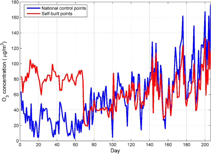
concentration in the air and the measurement error of the micro air quality detector15,30. Because too much sample data is not conducive to visually analyzing the change trend of air

pollutant concentration and the measurement error of the micro air quality detector, we calculated the daily average of the O3 concentration. After the data were averaged, a total of 206

sets of data were obtained31. It can be seen from Fig. 1 that the O3 concentration of the self-built point and the national control point are in good agreement in the later period, but there

is a certain deviation in the previous period. The low temperature and huge changes in humidity in autumn and winter interfere with the electrochemical sensor, which leads to deviations in

the measurement data of the micro air quality detector. In addition, the obvious difference in O3 concentration in different time periods can also be seen from Fig. 1. In order to visually

reflect the difference of O3 concentration in different time periods, this paper draws a box plot of O3 concentration changes with months. Figure 2 shows that the highest O3 concentration is

in June, and the lowest O3 concentration is in December (no data from July to October). O3 pollution has obvious seasonal characteristics32. Near-ground ozone is mostly generated by the

secondary conversion of nitrogen oxides and volatile organic compounds under high temperature and strong light conditions. The strong solar radiation and high temperature in summer can

easily cause photochemical smog and secondary ozone production. Continuous high temperature and strong sunshine weather is conducive to atmospheric photochemical reaction of nitrogen oxides

and volatile organic compounds, thereby generating strong oxidants such as near-ground ozone. Therefore, the O3 concentration in summer will increase as the temperature rises. CORRELATION

ANALYSIS Correlation mainly describes a potential relationship between two attributes. This relationship measures the degree to which one attribute contains the other. For the attribute of

numerical value, the commonly used measure of correlation is the correlation coefficient. Correlation coefficients are divided into Pearson correlation coefficients, Spearman correlation

coefficients and so on according to the applicable data types. The Pearson correlation coefficient measures the degree of linear correlation between two continuous numerical attributes, and

the Spearman correlation coefficient mainly describes the degree of correlation between hierarchical or ordered attributes. In this paper, the Pearson correlation coefficient (Eq. 1) is

selected as the evaluation index to measure the correlation between various pollutants and meteorological parameters. The absolute value of the correlation coefficient is between [0, 1]. An

absolute value of 0 indicates that the two attributes are completely unrelated, and an absolute value of 1 indicates that the two attributes are completely related. The larger the absolute

value of the correlation coefficient, the stronger the correlation. It can be seen from Table 2 that among the 11 variables, only the NO2 concentration and temperature are not significantly

correlated, and there is a significant correlation between the other variables. Figure 3 is a scatter plot of correlations between various variables. From the diagonal frequency histogram,

it can be seen that the concentrations of the six types of pollutants all present a right-skewed distribution, indicating that extreme weather with high pollutant concentrations often occurs

in this area. Most of the scatter plots between different variables are near a straight line, indicating that there is a certain linear correlation between them. $$r = \frac{{\mathop \sum

\nolimits_{i = 1}^{n} (x_{i} - \overline{x})\left( {y_{i} - \overline{y}} \right)}}{{\sqrt {\mathop \sum \nolimits_{i = 1}^{n} (x_{i} - \overline{x})^{2} } \cdot \sqrt {\mathop \sum

\nolimits_{i = 1}^{n} (y_{i} - \overline{y})^{2} } }}$$ (1) ESTABLISHMENT OF SENSOR CALIBRATION MODEL INTRODUCTION TO BASIC PRINCIPLES The classical least square estimation has been widely

used due to its many excellent properties. With the development of electronic computing technology, more and more accumulated experience in dealing with large-scale regression problems show

that the results obtained by least square estimation are sometimes very unsatisfactory. When the design matrix \(X\) is ill-conditioned, there is a strong linear correlation between the

column vectors of \(X\), that is, there is serious multicollinearity between the independent variables. In this case, using ordinary least squares to estimate the model parameters, the

variance of the parameters obtained is too large, and the effect of ordinary least squares becomes very unsatisfactory. Aiming at the problem that the ordinary least squares method obviously

deteriorates when multicollinearity occurs, the American scholar Hoerl proposed an improved least squares estimation method called ridge estimation in 1962. Later Hoerl and Kennard made a

systematic discussion in 197033. When there is multicollinearity between the independent variables, then \(\left| {X^{\prime}X} \right| \approx 0\). We add a matrix \(kI(k > 0)\) to

\(X^{\prime}X\), then the degree to which matrix \(X^{\prime}X + kI\) is close to singularity will be much smaller than the degree to which matrix \(X^{\prime}X\) is close to singularity.

Taking into account the dimension of variables, this article first standardizes the data. For the convenience of writing, the standardized design matrix is still denoted by \(X\). Equation 

(2) is defined as the ridge regression estimation of \(\beta\), where \(k\) is called the ridge parameter. Since \(X\) is assumed to have been standardized, \(X^{\prime}X\) is the sample

correlation matrix of the independent variables. \(\hat{\beta }\left( k \right)\) as the estimate of \(\beta\) is more stable than the least square estimation \(\hat{\beta }\). When \(k =

0\), the ridge estimation \(\hat{\beta }\left( 0 \right)\) is the ordinary least square estimation. Because the ridge parameter \(k\) is not unique, the ridge regression estimate

\(\hat{\beta }\left( k \right)\) is actually an estimated family of the regression parameter \(\beta\). For the selection of the ridge parameter \(k\), the commonly used methods include the

ridge trace method and the variance inflation factor method. $$\hat{\beta }\left( k \right) = \left( {X^{\prime}X + kI} \right)^{ - 1} X^{\prime}y$$ (2) The XGBoost algorithm is based on an

integrated learning method. The integrated learning method combines multiple learning models so that the combined model has stronger generalization ability to obtain better modeling effects.

XGBoost is an improvement on the boosting algorithm based on the gradient descent tree. It is composed of multiple decision tree iterations. XGBoost first builds multiple CART

(Classification and Regression Trees) models to predict the data set, and then integrates these trees as a new tree model. The model will continue to iteratively improve, and the new tree

model generated in each iteration will fit the residual of the previous tree. As the number of trees increases, the complexity of the ensemble model will gradually increase until it

approaches the complexity of the data itself, at which point the training achieves the best results. Equation (3) is the XGBoost algorithm model, where \(f_{t} \left( {x_{i} } \right) =

\omega_{q} \left( x \right)\) is the space of CART, \(\omega_{q} \left( x \right)\) is the score of sample \(x\), the model prediction value is obtained by accumulation, and q represents the

structure of each tree , \(T\) is the number of trees, and each \(f_{t}\) corresponds to an independent tree structure q and leaf weight. $$\hat{y}_{i} = \varphi \left( {x_{i} } \right) =

\mathop \sum \limits_{t = 1}^{T} f_{t} \left( {x_{i} } \right)$$ (3) XGBoost internal decision tree uses regression tree. For the squared loss function, the split node of the regression tree

fits the residual. For the general loss function (gradient descent), the split node of the regression tree fits the approximate value of the residual. Therefore, the accuracy of XGBoost

will be higher. Equations (4)–(7) are the iterative process of residual fitting. In Eq. (7), \(\hat{y}_{i}^{{\left( {t - 1} \right)}}\) is the predicted value of the i-th sample after t-1

iterations. \(\hat{y}_{i}^{\left( 0 \right)}\) is the initial value of the i-th sample. $$\hat{y}_{i}^{\left( 0 \right)} = 0$$ (4) $$\hat{y}_{i}^{\left( 1 \right)} = f_{1} \left( {x_{i} }

\right) = \hat{y}_{i}^{\left( 0 \right)} + f_{1} \left( {x_{i} } \right)$$ (5) $$\hat{y}_{i}^{\left( 2 \right)} = f_{1} \left( {x_{i} } \right) + f_{2} \left( {x_{i} } \right) =

\hat{y}_{i}^{\left( 1 \right)} + f_{2} \left( {x_{i} } \right)$$ (6) $$\hat{y}_{i}^{\left( t \right)} = \mathop \sum \limits_{k = 1}^{T} f_{k} \left( {x_{i} } \right) = \hat{y}_{i}^{{\left(

{t - 1} \right)}} + f_{t} \left( {x_{i} } \right)$$ (7) The objective optimization function of the XGBoost algorithm, that is, the loss function (Eq. 8), can be obtained according to the

iterative process of the residuals. For the general loss function, XGBoost will perform a second-order Taylor expansion in order to dig out more information about the gradient, and at the

same time remove the constant term, so that the gradient descent method can be better trained. Equations (9) and (10) are the loss function of the t-th step, where \(g_{i}\) and \(h_{i}\)

are the first and second derivatives. $$f_{obj}^{t} = \mathop \sum \limits_{i = 1}^{n} l\left( {y_{i} ,\hat{y}_{i}^{\left( t \right)} } \right) + \mathop \sum \limits_{i = 1}^{t} \Omega

\left( {f_{i} } \right) = \hat{y}_{i}^{{\left( {t - 1} \right)}} + f_{t} \left( {x_{i} } \right) = \mathop \sum \limits_{i = 1}^{n} l\left( {y \cdot \hat{y}_{i}^{\left( t \right)} } \right)

+ \Omega \left( {f_{i} } \right) + C$$ (8) $$g_{i} = \partial_{{\hat{y}_{i}^{{\left( {t - 1} \right)}} }} l\left( {y_{i} ,\hat{y}_{i}^{{\left( {t - 1} \right)}} } \right)$$ (9) $$h_{i} =

\partial_{{\hat{y}_{i}^{{\left( {t - 1} \right)}} }}^{2} l\left( {y_{i} ,\hat{y}_{i}^{{\left( {t - 1} \right)}} } \right)$$ (10) $$\Omega \left( f \right) = \gamma T + \frac{1}{2}\lambda

\mathop \sum \limits_{i = 1}^{n} \omega_{j}^{2}$$ (11) Different from other algorithms, the XGBoost algorithm adds a regularization term \(\Omega \left( f \right)\) (Eq. (11)) to prevent

over-fitting and better improve the accuracy of the model. \(\Omega \left( f \right)\) is a function that represents the complexity of the tree. The smaller the function value, the stronger

the generalization ability of the tree. \(\omega_{j}\) is the weight on the j-th leaf node in the tree f, \(T\) is the total number of leaf nodes in the tree, \({\upgamma }\) is the penalty

term of the L1 regularity, and \({\uplambda }\) is the penalty term of the L2 regularity, which is the custom parameter of the algorithm. Therefore, the objective function (Eqs. (12)–(14))

are obtained, where \(I_{j} = \left\{ {\left. i \right|q\left( {x_{i} } \right) = j} \right\}\) represents the sample set on the j-th leaf node28,34. $$f_{obj} = - \frac{1}{2}\mathop \sum

\limits_{j = 1}^{T} \frac{{G_{j}^{2} }}{{H_{j} + \lambda }} + \gamma T$$ (12) $$G_{j} = \mathop \sum \limits_{{i \in I_{j} }} g_{i}$$ (13) $$H_{j} = \mathop \sum \limits_{{i \in I_{j} }}

h_{i}$$ (14) RIDGE REGRESSION MODEL CONSTRUCTION Classical least squares estimation is often used to build pollutant concentration prediction models. It can also derive the quantitative

relationship between the various influencing factors and the concentration of pollutants15. However, the factors that affect the concentration of pollutants are more complicated, and through

the previous correlation analysis, it can be seen that there is a significant correlation between them. If the multiple linear regression model is directly established, multicollinearity

will be generated, which will cause the model's regression coefficients to be very unstable, and the model application ability will deteriorate. Ridge regression is often used to solve

the problem of model multicollinearity. We take the national control point O3 as the dependent variable, the pollutant concentration and meteorological parameters measured at the self-built

point as the independent variables, and establish a ridge regression model with the help of SPSS (Version20.0,https://www.ibm.com/cn-zh/analytics/spss-statistics-software). In this paper,

the ridge trace method is used to select the independent variables introduced into the model and the ridge parameter \(k\). In Fig. 4, the abscissa represents the value of the ridge

parameter \(k\), and each curve represents the standardized ridge regression coefficient of each variable. It can be seen that \(x_{4}\), \(x_{6}\), and \(x_{10}\) have relatively stable

ridge regression coefficients with relatively small absolute values, indicating that these variables have a small impact on the O3 concentration, and they can be deleted in the actual

modeling. In addition, although the standardized ridge regression coefficient of \(x_{2}\) is not small, it is very unstable, and rapidly tends to zero as \(k\) increases. For this kind of

variable whose ridge regression coefficient is not stable and the rapid vibration tends to zero, it can also be eliminated in the ridge regression model. After completing the selection of

the independent variables of the ridge regression model, the next step is the selection of the ridge parameter \(k\). We reduce the step length of the ridge parameter \(k\) to 0.02, and draw

the ridge trace diagram of the remaining variables as Fig. 5. It can be seen that when the ridge parameter \(k = 0.2\), the ridge trace of each variable is relatively stable, and the

coefficient of determination _R_2 is not reduced much, so the ridge parameter \(k = 0.2\) can be selected. Finally, with the help of SPSS software, use the selected variables and ridge

parameters to make a ridge regression model. Table 3 shows the unstandardized ridge regression equations for six types of pollutants. Using these equations, the predicted value of the ridge

regression model for the concentration of each pollutant can be obtained. RR-XGBOOST MODEL CONSTRUCTION The ridge regression model can be used to predict the concentration of pollutants, and

it can also show the quantitative relationship of the influence of each input variable on the concentration of pollutants. However, ridge regression can only show the linear relationship

between variables, while the nonlinear relationship between various factors and pollutant concentration has not been found. This study uses the ridge regression prediction value and

self-built point measurement data as input, and uses the pollutant concentration value monitored by the national control point as the output. The XGBoost algorithm is used to establish a

prediction model for the concentration of each pollutant. We call this model the RR-XGBoost model. Figure 6 is the flux diagram of the RR-XGBoost model. Before constructing the Ridge-XGBoost

model, first divide all samples into training set and test set randomly at a ratio of 8:2 (the other 5 pollutants data sets are also divided in the same way), and normalize all data to the

range of [0,1] based on experience29,34. The modeling in this paper is implemented using Python language programming, the simulation platform is Pycharm, and the Grid Search Method (GSM) is

used to find the optimal parameter combination. The XGBoost model has many parameters. If all parameters are optimized, the computer's memory will be challenged and the optimization

time will be greatly increased. In this paper, the following four main parameters are selected for optimization: (i) the number of gradient boosted trees n_estimators, the larger the

parameter, the better, but the occupied memory and training time will also increase accordingly, the optimization range of this article is 100–300; (ii) the maximum tree depth for base

learners max_depth, this parameter is used to avoid overfitting, the value range is 3–10; (iii) learning rate learning_rate, the value range is 0.01–0.3; and (iv) the minimum sum of instance

weight(hessian) needed in a child min_child_weight, which is similar to max_depth, used to avoid over-fitting, and the value range is 1–9. The four initial parameters of the XGBoost model

are set to 100, 6, 0.1, and 1. In addition, GSM needs to set the optimization step distance of each parameter during the optimization process (this article takes 10, 1, 0.01, 1). Table 4

shows the parameters of the XGBoost model determined after using the grid search method. In order to show the fitting effect of the RR-XGBoost model more intuitively, this paper draws the

fitting effect of O3 concentration as shown in Fig. 7. It can be seen that the correlation coefficient between the true concentration of O3 and the predicted concentration of the model in

both the training set and the test set exceeds 0.95. In addition, the regression coefficients of the two regression models (training set regression model and test set regression model) are

close to 1, indicating that this model performs well in predicting the concentration of pollutants. Figure 8 is the residual analysis diagram of the RR-XGBoost model. It can be seen that

most of the residual values of the model are randomly distributed within [-40, 40]. From the residual distribution histogram, it can be seen that the residuals are uniformly distributed

around zero, and the residuals are roughly normally distributed as a whole. DISCUSSION In order to further evaluate the prediction accuracy of the RR-XGBoost model, multilayer perceptron

neural network, random forest regression and support vector machine were used to compare with this model. This study uses four commonly used evaluation indicators to compare each model. The

four evaluation indicators are relative Mean Absolute Percent Error (MAPE), Mean Absolute Error (MAE), goodness of fit (_R_2), and Root Mean Square Error (RMSE) (Eqs. (15)–(18)). From Tables

5, 6, 7, and 8, it can be seen that the measurement accuracy of self-built points is the lowest among all evaluation indicators, which shows that the measurement accuracy of the micro air

quality detector needs to be improved. Although ridge regression can give the quantitative relationship between each variable and the concentration of pollutants, the fitting effect is not

particularly good. Random forest regression and XGBoost prediction methods are better in the accuracy of pollutant concentration prediction. In particular, the XGBoost prediction method can

greatly improve the accuracy of pollutant concentration prediction. The model combining ridge regression and XGBoost algorithm presented in this study is not only slightly higher in accuracy

than the single XGBoost prediction method, but also retains the advantages of ridge regression model. $$MAPE = \frac{1}{n}\mathop \sum \limits_{t = 1}^{n} \left| {\frac{{y_{t} - w_{t}

}}{{y_{t} }}} \right|$$ (15) $$MAE = \frac{1}{n}\mathop \sum \limits_{t = 1}^{n} \left| {y_{t} - w_{t} } \right|$$ (16) $$R^{2} = 1 - \frac{{\mathop \sum \nolimits_{t = 1}^{n} \left( {y_{t}

- w_{t} } \right)^{2} }}{{\mathop \sum \nolimits_{t = 1}^{n} \left( {y_{t} - \overline{y}} \right)^{2} }}$$ (17) $$RMSE = \sqrt {\frac{1}{n}\mathop \sum \limits_{t = 1}^{n} \left( {y_{t} -

w_{t} } \right)^{2} }$$ (18) Human activities are one of the important factors affecting the concentration of pollutants. Human activities have obvious periodic laws. We choose one week as a

cycle to evaluate the correction ability of the RR-XGBoost model to the measurement data of the micro air quality detector35. The blue curve in Fig. 9 is the measured value of the national

control point, the red curve is the measured value of the self-built point, and the black curve is the predicted value of the RR-XGBoost model. It can be seen that the red curve and the blue

curve have a certain error, but the black curve and the blue curve basically overlap, indicating that the RR-XGBoost model has performed a good correction on the measurement data of the

micro air quality detector. CONCLUSIONS Today, the situation of air pollution is still not very optimistic3, and atmospheric monitoring is gradually developing in the direction of refined

monitoring. At present, the most feasible solution for refined atmospheric monitoring is grid-based monitoring, that is, multiple air quality monitoring devices are set up within a certain

distance or range in a monitoring area to measure the specific dust particle concentration and pollutant gas concentration. A city will set up dozens to hundreds of monitoring points.

Accurate and fine grid air monitoring can quickly perceive and locate pollution events, and timely take control measures to achieve a multiplier control and governance effect5,7. At present,

many places use such micro-stations for the detection and law enforcement of sudden pollution situations, and even rank, reward and punish the air quality in the jurisdiction. Therefore,

higher requirements are put forward for the stability and accuracy of the micro air quality inspection station. With the development of computer technology, machine learning has entered the

latest stage, and machine learning has been more widely used in air quality prediction. The XGBoost algorithm is widely used in data modeling due to its excellent computational efficiency

and prediction accuracy. Unlike the random forest assigning the same voting weight to each decision tree, the generation of the next decision tree in the XGBoost algorithm is related to the

training and prediction of the previous decision tree. The XGBoost algorithm gives higher learning weights to the sample which has lower accuracy in the previous round of decision tree

training. Therefore, its accuracy is generally higher than the random forest algorithm. Compared with other ensemble learning algorithms, XGBoost improves the robustness of the model by

introducing regular terms and column sampling methods. On the other hand, it adopts a parallelization strategy when each tree chooses the split point, which greatly improves the speed of the

model. The combined model of ridge regression and XGBoost algorithm given in this paper can not only explain the quantitative relationship between input variables and output variables, but

also has certain advantages over other commonly used air quality monitoring models in terms of model accuracy. A total of 4135 samples were introduced into the Ridge-XGBoost model, and the

sample time spanned 4 seasons (206 days), which showed that the model performed well in terms of stability. Using the RR-XGBoost model to calibrate the data of the micro air quality detector

can make up for the shortcomings of the data monitoring accuracy of the micro air quality detector. The model plays an active role in the deployment of micro air quality detectors and grid

monitoring of the atmosphere. In future research, we can consider introducing more data to explore the evolution of pollutant concentrations on a larger time scale. In addition, in terms of

finding the optimal parameters, the grid search algorithm used in this study is not efficient enough when there are many parameters. We can try to find a more efficient parameter

optimization method to introduce more parameters to the model to further improve the accuracy of the model. REFERENCES * Qiu, H. _et al._ Machine learning approaches to predict peak demand

days of cardiovascular admissions considering environmental exposure. _Bmc. Med. Inform. Decis._ 1, 1–11 (2020). Google Scholar  * Corrigan, A. E., Becker, M. M., Neas, L. M., Cascio, W. E.

& Rappold, A. G. Fine particulate matters: The impact of air quality standards on cardiovascular mortality. _Environ. Res._ 161, 364–369 (2018). Article  CAS  Google Scholar  * Brauer,

M. _et al._ Exposure assessment for estimation of the global burden of disease attributable to outdoor air pollution. _Environ. Sci. Technol._ 46, 652–660 (2012). Article  ADS  CAS  Google

Scholar  * Akimoto, H. Global air quality and pollution. _Science_ 302, 1716–1719 (2004). Article  ADS  Google Scholar  * Castell, N. _et al._ Can commercial low-cost sensor platforms

contribute to air quality monitoring and exposure estimates?. _Environ. Int._ 99, 293–302 (2017). Article  CAS  Google Scholar  * Suárez Sánchez, A., García Nieto, P. J., Riesgo Fernández,

P., del Coz Díaz, J. J. & Iglesias-Rodríguez, F. J. Application of an SVM-based regression model to the air quality study at local scale in the Avilés urban area (Spain). _Math. Comput.

Model._ 54, 1453–1466 (2011). Article  Google Scholar  * Spinelle, L., Gerboles, M., Villani, M. G., Aleixandre, M. & Bonavitacola, F. Field calibration of a cluster of low-cost

available sensors for air quality monitoring. Part A: Ozone and nitrogen dioxide. _Sensor. Actuators B._ 215, 249–257 (2015). Article  CAS  Google Scholar  * Jian, L., Zhao, Y., Zhu, Y.,

Zhang, M. & Bertolatti, D. An application of ARIMA model to predict submicron particle concentrations from meteorological factors at a busy roadside in Hangzhou, China. _Sci. Total

Environ._ 426, 336–345 (2012). Article  ADS  CAS  Google Scholar  * Koo, J. W. _et al._ Prediction of Air Pollution Index in Kuala Lumpur using fuzzy time series and statistical models.

_Air. Qual. Atmos. Health._ 13, 77–88 (2019). Article  Google Scholar  * Lu, C. _et al._ Chemical composition of fog water in Nanjing area of China and its related fog microphysics. _Atmos.

Res._ 97, 47–69 (2010). Article  CAS  Google Scholar  * Tai, A. P. K., Mickley, L. J. & Jacob, D. J. Correlations between fine particulate matter (PM2.5) and meteorological variables in

the United States: Implications for the sensitivity of PM2.5 to climate change. _Atmos. Environ._ 44, 3976–3984 (2010). Article  ADS  CAS  Google Scholar  * Azid, A. _et al._ Assessing

indoor air quality using chemometric models. _Pol. J. Environ. Stud._ 6, 2443–2450 (2018). Article  Google Scholar  * Liu, B., Zhao, Q., Jin, Y., Shen, J. & Li, C. Application of

combined model of stepwise regression analysis and artificial neural network in data calibration of miniature air quality detector. _Sci. Rep-UK_ 11, 1–12.

https://doi.org/10.1038/s41598-021-82871-4 (2021). Article  ADS  CAS  Google Scholar  * Elbayoumi, M., Ramli, N. A. & Faizah, F. M. Y. N. Development and comparison of regression models

and feedforward backpropagation neural network models to predict seasonal indoor PM2.5–10 and PM2.5 concentrations in naturally ventilated schools. _Atmos. Pollut. Res._ 6, 1013–1023 (2015).

Article  Google Scholar  * Huang, Z. & Zhang, R. Efficient estimation of adaptive varying-coefficient partially linear regression model. _Stat. Probab. Lett._ 79, 943–952 (2009).

Article  MathSciNet  Google Scholar  * Samia, A., Kaouther, N. & Abdelwahed, T. A hybrid ARIMA and artificial neural networks model to forecast air quality in urban areas: Case of

Tunisia. _Adv. Mater._ 518, 2969–2979 (2012). Google Scholar  * Elangasinghe, M. A., Singhal, N., Dirks, K. N., Salmond, J. A. & Samarasinghe, S. Complex time series analysis of PM10 and

PM2.5 for a coastal site using artificial neural network modelling and k-means clustering. _Atmos. Environ._ 94, 106–116 (2014). Article  ADS  CAS  Google Scholar  * Wang, Z., Feng, J., Fu,

Q. & Gao, S. Quality control of online monitoring data of air pollutants using artificial neural networks. _Air Qual. Atmos. Health._ 12, 1189–1196 (2019). Article  CAS  Google Scholar

  * Sun, W. _et al._ Prediction of 24-hour-average pm2.5 concentrations using a hidden Markov model with different emission distributions in Northern California. _Sci. Total Environ._ 443,

93–103 (2013). Article  ADS  CAS  Google Scholar  * Oettl, D., Almbauer, R. A., Sturm, P. J. & Pretterhofer, G. Dispersion modelling of air pollution caused by road traffic using a

Markov chain–Monte Carlo model. _Stoch. Environ. Res. Risk Assess._ 17, 58–75 (2003). Article  Google Scholar  * Dong, M. _et al._ PM2.5 concentration prediction using hidden semi-Markov

model-based times series data mining. _Expert. Syst. Appl._ 36, 9046–9055 (2009). Article  Google Scholar  * Liu, B. _et al._ Urban air quality forecasting based on multi-dimensional

collaborative Support Vector Regression (SVR): A case study of Beijing-Tianjin-Shijiazhuang. _PLoS ONE_ 7, 1–17 (2017). Google Scholar  * Zhu, S. _et al._ PM2.5 forecasting using SVR with

PSOGSA algorithm based on CEEMD, GRNN and GCA considering meteorological factors. _Atmos. Environ._ 183, 20–32 (2018). Article  ADS  CAS  Google Scholar  * Liu, B., Jin, Y. & Li, C.

Analysis and prediction of air quality in Nanjing from autumn 2018 to summer 2019 using PCR-SVR-ARMA combined model. _Sci. Rep-UK_ 11, 1–14. https://doi.org/10.1038/s41598-020-79462-0

(2021). Article  ADS  CAS  Google Scholar  * Zimmerman, N. _et al._ A machine learning calibration model using random forests to improve sensor performance for lower-cost air quality

monitoring. _Atmos. Meas. Tech._ 11, 291–313 (2018). Article  Google Scholar  * Ding, H. J., Liu, J. Y., Zhang, C. M. & Wang, Q. Predicting optimal parameters with random forest for

quantum key distribution. _Quantum Inf. Process._ 2, 1–8 (2020). MathSciNet  Google Scholar  * Kamińska, J. A. The use of random forests in modelling short-term air pollution effects based

on traffic and meteorological conditions: A case study in Wrocaw. _J. Environ. Manage._ 217, 164–174 (2018). Article  Google Scholar  * Zhai, B. & Chen, J. Development of a stacked

ensemble model for forecasting and analyzing daily average PM2.5 concentrations in Beijing, China. _Sci. Total Environ._ 635, 644–658 (2018). Article  ADS  CAS  Google Scholar  *

Joharestani, M. Z., Cao, C., Ni, X., Bashir, B. & Talebiesfandarani, S. PM2.5 prediction based on Random Forest, XGBoost, and deep learning using multisource remote sensing data.

_Atmosphere_ 10, 373 (2019). Article  ADS  Google Scholar  * Cordero, J. M., Borge, R. & Narros, A. Using statistical methods to carry out in field calibrations of low cost air quality

sensors. _Sens. Actuators B_ 267, 245–254 (2018). Article  CAS  Google Scholar  * Liu, Q., Liu, Y., Yang, Z., Zhang, T. & Zhong, Z. Daily variations of chemical properties in airborne

particulate matter during a high pollution winter episode in Beijing. _Acta Sci. Circumst._ 34, 12–18 (2014). CAS  Google Scholar  * Wang, X. & Lu, W. Seasonal variation of air pollution

index: Hong Kong case study. _Chemosphere_ 63, 1261–1272 (2006). Article  ADS  CAS  Google Scholar  * Huang, D., Guan, P., Guo, J., Wang, P. & Zhou, B. Investigating the effects of

climate variations on bacillary dysentery incidence in northeast China using ridge regression and hierarchical cluster analysis. _BMC Infect. Dis._ 8, 130 (2008). Article  Google Scholar  *

Duen-Ren, L., Shin-Jye, L., Huang, Y. & Chien-Ju, C. Air pollution forecasting based on attention-based LSTM neural network and ensemble learning. _Expert Syst._ 3, 1–16 (2020). Google

Scholar  * Lei, M. T., Monjardino, J., Mendes, L. & Ferreira, F. Macao air quality forecast using statistical methods. _Air. Qual. Atmos. Health._ 2, 249–258 (2019). Google Scholar 

Download references ACKNOWLEDGEMENTS This work was supported by the Youth Program of National Natural Science Foundation of China (No.71602051) and Research Project of Higher Vocational

Education in Nanjing Vocational University of Industry Technology (No. GJ20-30). AUTHOR INFORMATION AUTHORS AND AFFILIATIONS * Public Foundational Courses Department, Nanjing Vocational

University of Industry Technology, Nanjing, 210023, China Bing Liu, Xianghua Tan & Yueqiang Jin * School of Mechanical Engineering, Nanjing Vocational University of Industry Technology,

Nanjing, 210023, China Wangwang Yu * College of Management, Henan University of Technology, Zhengzhou, 450001, China Chaoyang Li Authors * Bing Liu View author publications You can also

search for this author inPubMed Google Scholar * Xianghua Tan View author publications You can also search for this author inPubMed Google Scholar * Yueqiang Jin View author publications You

can also search for this author inPubMed Google Scholar * Wangwang Yu View author publications You can also search for this author inPubMed Google Scholar * Chaoyang Li View author

publications You can also search for this author inPubMed Google Scholar CONTRIBUTIONS B.L., X.T., Y.J. and W.Y. wrote the main manuscript text, and C.L. is responsible for data processing

and model verification. CORRESPONDING AUTHOR Correspondence to Bing Liu. ETHICS DECLARATIONS COMPETING INTERESTS The authors declare no competing interests. ADDITIONAL INFORMATION

PUBLISHER'S NOTE Springer Nature remains neutral with regard to jurisdictional claims in published maps and institutional affiliations. RIGHTS AND PERMISSIONS OPEN ACCESS This article

is licensed under a Creative Commons Attribution 4.0 International License, which permits use, sharing, adaptation, distribution and reproduction in any medium or format, as long as you give

appropriate credit to the original author(s) and the source, provide a link to the Creative Commons licence, and indicate if changes were made. The images or other third party material in

this article are included in the article's Creative Commons licence, unless indicated otherwise in a credit line to the material. If material is not included in the article's

Creative Commons licence and your intended use is not permitted by statutory regulation or exceeds the permitted use, you will need to obtain permission directly from the copyright holder.

To view a copy of this licence, visit http://creativecommons.org/licenses/by/4.0/. Reprints and permissions ABOUT THIS ARTICLE CITE THIS ARTICLE Liu, B., Tan, X., Jin, Y. _et al._

Application of RR-XGBoost combined model in data calibration of micro air quality detector. _Sci Rep_ 11, 15662 (2021). https://doi.org/10.1038/s41598-021-95027-1 Download citation *

Received: 02 March 2021 * Accepted: 20 July 2021 * Published: 02 August 2021 * DOI: https://doi.org/10.1038/s41598-021-95027-1 SHARE THIS ARTICLE Anyone you share the following link with

will be able to read this content: Get shareable link Sorry, a shareable link is not currently available for this article. Copy to clipboard Provided by the Springer Nature SharedIt

content-sharing initiative