A practical solution of the bethe equation in the energy range applicable to radiotherapy and radionuclide production

ABSTRACT While the dose deposition of charged hadrons has received much attention over the last decades starting in 1930 with the publication of the Bethe equation, there are still practical

obstacles in implementing it in fields like radiotherapy and isotope production on cyclotrons. This is especially true if the target material consists of non-homogeneous materials, either

consisting of a mixture of different elements or experiencing phase changes during irradiation. While Monte-Carlo methods have had great success in describing these more difficult target

materials, they come at a computational cost, especially if the problem is time-dependent. This can greatly hinder optimal advancement in therapy and isotope targetry. Here, a regular

perturbation method is used to solve the Bethe equation in the limit of small relativistic effects. Particular focus is given to incident energy level relevant to radionuclide production and

radiotherapy applications, i.e. 10–200 MeV. We present a series solution for the range and dose distribution in terms of elementary functions, as opposed to special functions which will aid

in uptake by practitioners. SIMILAR CONTENT BEING VIEWED BY OTHERS NON-LINEAR QED APPROACH FOR BETATRON RADIATION IN A LASER WAKEFIELD ACCELERATOR Article Open access 05 January 2024 FUTURE

DIRECTIONS ON LOW-ENERGY RADIATION DOSIMETRY Article Open access 19 May 2021 OPTIMIZING FOCUSED VERY-HIGH-ENERGY ELECTRON BEAMS FOR RADIATION THERAPY BASED ON MONTE CARLO SIMULATION Article

Open access 11 November 2024 INTRODUCTION Charged hadrons, like ions or more commonly protons, are an increasingly important tool in both radiotherapy, to treat cancer, and in radioisotope

production for use in nuclear medicine applications. Currently there are 94 hadron-therapy centers in operation worldwide, with 66 more under construction or in the planning stages1, and

more than 1270 cyclotrons are currently used for the production of radioisotopes2. Understanding the interaction of protons with matter is therefore not restricted to the understanding of

fundamental mechanisms, but has also wide-ranging implications for health care3,4. Protons differ from photons in how they lose energy while traveling through matter. Charged protons lose

energy continuously, mainly through ionization of the atoms of the matter they are traversing. The energy loss per unit distance in the non-relativistic regime was described by Bethe5. At

the end of their range, before the protons come to rest, the interaction cross–section increases as the proton velocity decreases. This results in the Bragg peak whose position is defined,

primarily, by the initial energy of the protons. Knowing this position accurately is crucial when treating cancer to avoid excessive dose to neighboring healthy tissue and to take full

advantage of the cell-killing properties of the protons. It is also important when designing targets for medical isotope production, as the Bragg peak coincides with the largest heat

deposition. This large localized power deposition, if not properly controlled, can increase the temperature and, in a closed system, the pressure in the target to the point of rupture,

leading to the release of radioactivity. While the range of protons in matter is tabulated for several materials6,7, it is still difficult to handle for mixed materials, for example

non-homogeneous tissue in patients or phase changes in targets. In these situations Monte-Carlo packages like SRIM8, FLUKA9,10, Geant411, MCNP12 and others, are often employed with great

success but also significant computational cost and time delay, slowing down development or clinical implementation. The average energy _E_ lost by the protons per unit distance _x_ while

traversing through matter is given by the Bethe equation5 as reported by Grimes _et al_.13 $$-\frac{dE}{dx}=\frac{4\pi n{z}^{2}}{{m}_{e}{c}^{2}{\beta }^{2}}{(\frac{{e}^{2}}{4\pi {\varepsilon

}_{o}})}^{2}(\mathrm{ln}(\frac{2{m}_{e}{c}^{2}{\beta }^{2}}{I(1-{\beta }^{2})})-{\beta }^{2})$$ (1) where _n_ is the electron density of the target material; _e_ is the electron charge;

_m__e_ is the electron mass; _I_ is the mean excitation potential of the target material; _z_ is the multiple of the electron charge of the projectile; \(\beta \equiv u/c\) is the ratio of

the projectile velocity to the speed of light in vacuum, _c_; and \({\varepsilon }_{0}\) is the vacuum permittivity. The Bethe equation is a result of a first-order Born approximation with

the projectile being faster than the bound electrons in the target atoms. The energy of a proton beam _E_ is related to the mass _m__p_ and velocity of a proton via $$E={m}_{p}{c}^{2}(\gamma

-1)\,\,\gamma ={(1-{\beta }^{2})}^{-1/2},$$ (2) and, with the use of the chain-rule, we find $$\frac{dE}{dx}={m}_{p}{\gamma }^{3}u\frac{du}{dx}$$ (3) from which we may express the Bethe

equation as $${\gamma }^{3}u\frac{{\rm{d}}u}{{\rm{d}}x}=-\,\frac{A}{{u}^{2}}(\mathrm{ln}(\frac{B{u}^{2}}{1-{\beta }^{2}})-{\beta }^{2}).$$ (4) Here, _A_ \(({m}^{3}/{s}^{4})\) and _B_

\(({s}^{2}/{m}^{2})\) are defined as $$A=\frac{4\pi n{z}^{2}}{{m}_{e}{m}_{p}}{(\frac{{e}^{2}}{4\pi {\varepsilon }_{o}})}^{2}\,\,B=\frac{2{m}_{e}}{I}$$ (5) with representative values for

common materials given in Table 1. The reduction given by Eqs. 2–5 was advanced by Grimes _et al_.13, which we use directly in this work. Using the continuous-slowing-down-approximation

(CSDA), Eq. 4 has been integrated from the projectiles’ initial velocity to its resting state using a number of different techniques in order to determine its range _R_, defined as the root

of \(u(R)=0\)8,14,15,16. Of note is a recent solution of the Bethe equation advanced by Grimes _et al_.13 who show that in the non-relativistic limit (\(\varepsilon \equiv {u}_{o}/c\to 0\))

$$\frac{RA}{{u}_{o}^{4}}=-\,\frac{1}{2{b}^{2}}{E}_{1}(\,-\,2\,\mathrm{ln}(b))+O({\varepsilon }^{2})\,\,(b\equiv B{u}_{o}^{2}\,{\rm{with}}\,b > 1)$$ (6) where _E_1 is the exponential

integral; _u__o_ is the initial velocity of the particles; _b_ is dimensionless and related to the ratio of the incident energy to the mean excitation potential; and the big-_O_ notation is

used to describe the error term in the approximation. It indicates that the absolute value of the error is approximately \({\varepsilon }^{2}\). We also note that the grouping on the

left-hand side of the equation is dimensionless indicating that the characteristic length \({\ell }_{c}\) for this problem is \({\ell }_{c}\equiv {u}_{o}^{4}/A\), as _R_ has units of length.

The third dimensionless group that governs this problem is \(\varepsilon \), the ratio of the particle velocity to the speed of light. This solution indicates that the (dimensionless) range

\(R/{\ell }_{c}\) may be uniquely expressed as a function of _b_ and \(\varepsilon \), and to lowest order is independent of relativistic effects. More importantly, this solution

methodology may be extended and used to estimate the dose distribution. However, to do so one requires the use of an inverse exponential integral function, a non-standard function, which

Grimes _et al_.13 indicate that no closed-form expression exists which hinders the utility of this expression. Overcoming this difficulty motivates this work. In this work, we present a

solution of the Bethe equation using a regular perturbation method. Using a solution methodology different to that performed by Grimes _et al_.13, we are able to create a reasonable solution

which avoids the use of the exponential integral. We present our solution in the small relativistic limit and then extend the number of terms to cover the energy range up to ~200 MeV for

protons. We find that with this novel solution the complexity of using the Bethe equation has been reduced dramatically, without significant loss of precision. Because of this, we anticipate

uptake of these expressions by the radioisotope and radiotherapy communities17 for optimization purposes, for example target design. MODEL DERIVATION Our methodology is inspired by Grimes

_et al_.13 who demonstrate that the problem can be approximated by a series solution. Here, we present an alternative methodology in creating the series and begin our solution by scaling Eq.

 4 with $${\boldsymbol{u}}=\frac{u}{{u}_{o}}\,\,({\boldsymbol{x}},{\boldsymbol{R}})=\frac{1}{{\ell }_{c}}(x,R)$$ (7) and then switch the roles of the dependent and independent variables to

avoid divergence of the velocity gradient near the Bragg peak. This yields $$\frac{{\rm{d}}{\boldsymbol{x}}}{{\rm{d}}{\boldsymbol{u}}}=-\,\frac{{{\boldsymbol{u}}}^{3}}{{(1-{(\varepsilon

{\boldsymbol{u}})}^{2})}^{3/2}}{(\mathrm{ln}(-\frac{b{{\boldsymbol{u}}}^{2}}{1-{(\varepsilon {\boldsymbol{u}})}^{2}})-{(\varepsilon {\boldsymbol{u}})}^{2})}^{-1}\equiv

{\mathfrak{F}}({\boldsymbol{u}}),\,\,{\boldsymbol{x}}(1)=0$$ (8) where \({\mathfrak{F}}({\boldsymbol{u}})\) can be approximated by a Taylor series about \(\varepsilon =0\), i.e.

$$\begin{array}{rcl}{\mathfrak{F}}({\boldsymbol{u}}) & = & -\frac{{{\boldsymbol{u}}}^{3}}{\mathrm{ln}(b{{\boldsymbol{u}}}^{2})}-{\varepsilon

}^{2}\frac{3{{\boldsymbol{u}}}^{5}}{2\,\mathrm{ln}\,(b{{\boldsymbol{u}}}^{2})}\\ & & -\,{\varepsilon

}^{4}\frac{{{\boldsymbol{u}}}^{7}}{\mathrm{ln}\,(b{{\boldsymbol{u}}}^{2})}(\frac{15}{8}-\frac{1}{2\,\mathrm{ln}\,(b{{\boldsymbol{u}}}^{2})})\\ & & -\,{\varepsilon

}^{6}\frac{{{\boldsymbol{u}}}^{9}}{\mathrm{ln}\,(b{{\boldsymbol{u}}}^{2})}(\frac{35}{16}-\frac{13}{12\,\mathrm{ln}\,(b{{\boldsymbol{u}}}^{2})})+O({\varepsilon }^{8})\end{array}$$ (9) If we

seek a solution of the form $${\boldsymbol{x}}({\boldsymbol{u}})={{\boldsymbol{x}}}_{o}({\boldsymbol{u}})+{\varepsilon }^{2}{{\boldsymbol{x}}}_{1}({\boldsymbol{u}})+{\varepsilon

}^{4}{{\boldsymbol{x}}}_{2}({\boldsymbol{u}})+{\varepsilon }^{6}{{\boldsymbol{x}}}_{3}({\boldsymbol{u}})+O({\varepsilon }^{8})$$ (10) and reduce the complexity of the notation by

transforming the dependent variable using $$z=-\,2\,\mathrm{ln}(b{{\boldsymbol{u}}}^{2})$$ (11) we find that $$\begin{array}{ll}O(1): &

\frac{{\rm{d}}{{\boldsymbol{x}}}_{0}}{{\rm{d}}z}=-\,\frac{1}{2{b}^{2}}\frac{{{\rm{e}}}^{-z}}{z}\end{array}$$ (12) $$\begin{array}{ll}O({\varepsilon }^{2}): &

\frac{{\rm{d}}{{\boldsymbol{x}}}_{1}}{{\rm{d}}z}=-\,\frac{3}{4{b}^{3}}\frac{{{\rm{e}}}^{-\frac{3z}{2}}}{z}\end{array}$$ (13) $$\begin{array}{ll}O({\varepsilon }^{4}): &

\frac{{\rm{d}}{{\boldsymbol{x}}}_{2}}{{\rm{d}}z}=-\,\frac{1}{16{b}^{4}}\frac{{{\rm{e}}}^{-2z}(15\,z+8)}{{z}^{2}}\end{array}$$ (14) $$\begin{array}{ll}O({\varepsilon }^{6}): &

\frac{{\rm{d}}{{\boldsymbol{x}}}_{3}}{{\rm{d}}z}=-\,\frac{{{\rm{e}}}^{-5/2z}(105\,z+104)}{96\,{b}^{5}{z}^{2}}\end{array}$$ (15) when terms of equal order are equated. Under this transform,

we note that at the stopping distance the transformed variable is unbounded, _i_._e_. \(z\to \infty \), as \({\boldsymbol{u}}\to 0\). Indeed, when the beam first enters the target

\({z}_{o}=-\,2\,\mathrm{ln}(b)\) as \({\boldsymbol{u}}(0)=1\). APPLICATIONS ESTIMATING RANGE We estimate the range by solving Eq. 12 as an example. Following this we simply report the

solution for the higher order terms, i.e. Eqs. 13 and 15. We begin by integrating Eq. 12 by parts to give $${\boldsymbol{R}}=-\,\frac{1}{2{b}^{2}}\,{\int }_{{z}_{o}}^{\infty

}\,\frac{{{\rm{e}}}^{-{\rm{z}}}}{z}dz=-\,\frac{1}{2{b}^{2}}({-\frac{{{\rm{e}}}^{-z}}{z}|}_{{z}_{o}}^{\infty }-{\int }_{{z}_{o}}^{\infty

}\,\frac{{{\rm{e}}}^{-z}}{{z}^{2}}dz)=-\,\frac{1}{2{b}^{2}}(\frac{{{\rm{e}}}^{-{z}_{o}}}{{z}_{o}}-{\int }_{{z}_{o}}^{\infty }\,\frac{{{\rm{e}}}^{-z}}{{z}^{2}}dz)+O({\varepsilon }^{2})$$ (16)

In an unmotivated trick, we do so so again and find that $${\boldsymbol{R}}=-\,\frac{1}{2{b}^{2}}(\frac{{{\rm{e}}}^{-{z}_{o}}}{{z}_{o}}-\frac{{{\rm{e}}}^{-{z}_{o}}}{{z}_{o}^{2}}+2\,{\int

}_{{z}_{o}}^{\infty }\,\frac{{{\rm{e}}}^{-z}}{{z}^{3}}dz)+O({\varepsilon }^{2})$$ (17) With this we postulate that the solution of the problem may be expressed as a series in 1/_z__o_ as the

magnitude of _z__o_ is large. When this integration procedure is repeated, we find that

$${\boldsymbol{R}}=-\,\frac{1}{2{b}^{2}}\frac{{e}^{-{z}_{o}}}{{z}_{o}}(1-\frac{1}{{z}_{o}}+\frac{2}{{z}_{o}^{2}}+\ldots )=-\,\frac{{e}^{-{z}_{o}}}{2{b}^{2}}\,\mathop{\sum

}\limits_{n=1}^{N}\,{(-1)}^{n+1}\frac{(n-1)!}{{z}_{o}^{n}}$$ (18) For insight into this series, we estimate the magnitude of the three first terms using helium as the target material and 100

 MeV protons as the projectiles. We estimate \(b=4.5\times {10}^{3}\) and \({z}_{0}=-\,16.8\), giving _i_._e_. \(-\,1/{z}_{0}=0.06\) and \(2/{z}_{0}^{2}=0.007\); hence \(1 < -\,1/{z}_{0}

< 2/{z}_{0}^{2}\), implying a convergent series. This solution may be expressed in a more convenient form by using Eq. 11. Indeed, we find that

$${\boldsymbol{R}}=\frac{2\,{\mathrm{ln}}^{2}\,b+\,\mathrm{ln}\,b-1}{8\,{\mathrm{ln}}^{3}\,b}$$ (19) when truncated after three terms, representing an error of ~1% at 100 MeV. We extend the

leading-order solution by repeating the procedure given above and solve Eqs. 13–15 using the same procedure to find that $$\begin{array}{rcl}{\boldsymbol{R}} & = &

(\frac{2\,{\mathrm{ln}}^{2}\,b+\,\mathrm{ln}\,b-1}{8\,{\mathrm{ln}}^{3}\,b})+{\varepsilon }^{2}(\frac{9\,{\mathrm{ln}}^{2}\,b-3\,\mathrm{ln}\,b+2}{36\,{\mathrm{ln}}^{3}\,b})\\ & &

+\,{\varepsilon }^{4}(\frac{120\,{\mathrm{ln}}^{2}\,b-2\,\mathrm{ln}\,b-1}{512\,{\mathrm{ln}}^{3}\,b})-31{\varepsilon

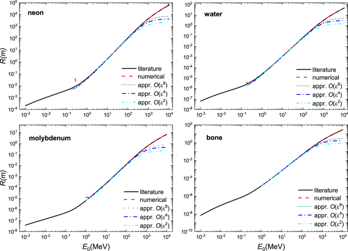
}^{6}(\frac{25\,{\mathrm{ln}}^{2}\,b+5\,\mathrm{ln}\,b+2}{2400\,{\mathrm{ln}}^{3}\,b})\end{array}$$ (20) We demonstrate the usefulness of this solution in Fig. 1 where excellent agreement is

found when compared to literature values7 and a numerical solution of the Bethe equation using Romberg integration by applying Richardson extrapolation on a trapezoidal rule for a select

number of materials - a gas, liquid, a solid and a complex material; a larger selection of material is shown in Figs. 2, 3 and 4. These calculations were performed using the parameters given

in Table 1. At \(O({\varepsilon }^{2})\) the solution is fairly reasonable to 50 MeV; at \(O({\varepsilon }^{8})\) the expression yields reasonable estimates to ~200 MeV. The immediate

benefit of Eq. 20 is that we are able to estimate the stopping distance without use of the exponential integral. Increasing the number of terms does not improve the fit below 1 MeV as the

Barkas and Bloch corrections are not included. Interestingly, we find that the empirical expression18,19 $$R=\alpha {E}_{0}^{p}$$ (21) behaves similarly to our solution. Here, _α_ is a

material dependent constant and _p_ depends on the proton velocity which typical ranges from 1.5 to 2. As can be seen in Fig. 5, in the region \({10}^{1} < b < {10}^{3}\), _R_ varies

only weakly implying that over small energy intervals, _R_ may be taken as constant, yielding \(R\propto {E}_{0}^{2}\). This is also evident if we solve the Bethe equation without including

the logarithmic term. ESTIMATING DOSE DISTRIBUTION To estimate the dose distribution _U_(_X_), we proceed in an analogous manner to that given above. Here, we examine the solution to the

leading order equation, i.e. Eq. 12 and then report the solution to the higher order terms. As Eq. 12 is separable, we are in a position to integrate this expression by parts, repeatedly, to

generate a series in 1/_z_. We abandon the initial condition (\({\boldsymbol{x}}({z}_{o})=0\)) and in its place, use the stopping condition defining the range,(\({\boldsymbol{x}}({z}_{o}\to

\infty )={\boldsymbol{R}}\)). By doing so, this dramatically aids in the evaluation of the integral and allows for the development of the series. To highlight this procedure, we rewrite Eq.

 12 as $${\int }_{{\boldsymbol{x}}}^{{\boldsymbol{R}}}\,d{\boldsymbol{x}}=-\,\frac{1}{2{b}^{2}}\,{\int }_{z}^{\infty }\,\frac{{{\rm{e}}}^{-z}}{z}dz+O({\varepsilon }^{2})$$ (22) which can be

integrated to give $${\boldsymbol{R}}-{\boldsymbol{x}}=-\,\frac{1}{2{b}^{2}}({-\frac{{{\rm{e}}}^{-z}}{z}|}_{z}^{\infty }-{\int }_{z}^{\infty

}\,\frac{{{\rm{e}}}^{-z}}{{z}^{2}}dz)=-\,\frac{1}{2{b}^{2}}(\frac{{{\rm{e}}}^{-z}}{z}-{\int }_{z}^{\infty }\,\frac{{{\rm{e}}}^{-z}}{{z}^{2}}dz)+O({\varepsilon }^{2})$$ (23) This is directly

analogous to the problem solved previously and allows us to write $${\boldsymbol{R}}-{\boldsymbol{x}}=-\,\frac{{e}^{-z}}{2{b}^{2}}\,\mathop{\sum

}\limits_{n=1}^{N}\,{(-1)}^{n+1}\frac{(n-1)!}{{z}^{n}}$$ (24) or

$${\boldsymbol{x}}-{\boldsymbol{R}}=-\,\frac{{{\boldsymbol{u}}}^{4}(2{(\mathrm{ln}(b{{\boldsymbol{u}}}^{2}))}^{2}+\,\mathrm{ln}(b{{\boldsymbol{u}}}^{2})+1)}{8{(\mathrm{ln}(b{{\boldsymbol{u}}}^{2}))}^{3}}$$

(25) when truncated after three terms. When this process is repeated and extended to the next term we find

$${\boldsymbol{x}}-{\boldsymbol{R}}=-\,\frac{{{\boldsymbol{u}}}^{4}(2{(\mathrm{ln}(b{{\boldsymbol{u}}}^{2}))}^{2}+\,\mathrm{ln}(b{{\boldsymbol{u}}}^{2})+1)}{8{(\mathrm{ln}(b{{\boldsymbol{u}}}^{2}))}^{3}}-{\varepsilon

}^{2}\frac{{{\boldsymbol{u}}}^{6}(9{(\mathrm{ln}(b{{\boldsymbol{u}}}^{2}))}^{2}+3\,\mathrm{ln}(b{{\boldsymbol{u}}}^{2})+2)}{36{(\mathrm{ln}(b{{\boldsymbol{u}}}^{2}))}^{3}}$$ (26) Finally,

we apply the solution methodology to the higher order terms as $$\begin{array}{ll}O({\varepsilon }^{4}): &

-\frac{(120{(\mathrm{ln}(b{{\boldsymbol{u}}}^{2}))}^{2}-2\,\mathrm{ln}(b{{\boldsymbol{u}}}^{2})-1){{\boldsymbol{u}}}^{8}}{512{(\mathrm{ln}(b{{\boldsymbol{u}}}^{2}))}^{3}}\end{array}$$ (27)

$$\begin{array}{ll}O({\varepsilon }^{6}): &

+\frac{31(25{(\mathrm{ln}(b{{\boldsymbol{u}}}^{2}))}^{2}+5\,\mathrm{ln}(b{{\boldsymbol{u}}}^{2})+2){{\boldsymbol{u}}}^{10}}{2400{(\mathrm{ln}(b{{\boldsymbol{u}}}^{2}))}^{3}}\end{array}$$

(28) A representative comparison is given in Fig. 6 where the numerical and approximate solution are compared to SRIM8 of the dose distribution of 100 MeV protons impinging in four different

materials. The data points are average energy results of protons intersecting the individual depth and the error bars are the corresponding standard deviations of the individual energy

spreads. Again, very good agreement is observed between the analytical and our approximate solution and with SRIM simulations. ROBUSTNESS OF THE SOLUTION In this work we present a series

solution to approximate the solution of the Bethe equation. We have tested the error in this approximation by comparison to a numerical solution, tabulated data, and SRIM calculations. We

find excellent agreement over a defined proton energy range applicable to radiotherapy and radionuclide production. One immediate benefit of this solution is that estimate

water-equivalent-thickness for radiotherapy applications can be improved, over the empirical Bragg-Kleemann law19. Care must be given in interpretation of our solution. In essence, we

advance a simpler solution to the Bethe equation. Although the Bethe equation is routinely used, there are limitations in its use. In practice, there are a number of physical mechanisms

which cause deviations from the range predicted by Eq. 6. As is evident in our results, the first type of deviations occurs at low incident energy, where the first-Born approximation reaches

its limit. Here we find corrections to the form of the Bethe equation by Barkas or Bloch6. In this energy regime the Barkas, Bloch and Shell correction need to be applied. In addition, at

high projectile energies, relativistic and density effects and radiative losses need to be taken into account6. In the second category, we find that the distance travelled by the particle

along its initial direction is slightly reduced by small deflections caused by scattering. The impact of this is minimal for low _Z_ materials, with the ‘detour factor’ of the projected

range greater than 99.87% for protons of energy >100 MeV in water6 or for metals where the stopping distance is small. Outside of this range, the detour factor becomes substantial,

especially for gases16 where Schlyer _et al_.20 shows that the standard deviation of the probability distribution in scattering angle is related in a complex manner to the local energy of

the beam. In the third category, we find a number of works highlighting the effect of a two-way coupling between the beam and the absorbing material on the irradiation profile. In perhaps

the most widely cited series of work, Heselius and his co-workers21,22 demonstrate experimentally symmetry-breaking in the beam profile when density of the gas target is stratified due to

localized heating. Indeed, this problem is relatively unexplored on the theoretical front with most authors de-coupling the temperature effects23,24,25,26. In perhaps the most comprehensive

study, O’Brien and her co-workers25,27,28 couples Monte-Carlo simulation of the beam profile with Reynolds-Averaged Navier-Stokes (RANS)29 modelling of the transport equations to estimate

the temperature, density and beam profile. Interestingly, with these latter two categories, these deviations are not evident in our result in this range, even with gas. CONCLUSION We present

a simple and easy to implement approximate solution of the Bethe equation with good agreement in the proton energy range of 10 MeV to approximately 200 MeV, applicable for the energy range

of proton radiotherapy and medical isotope production. Although tabulated values are available for uniform materials, this solution methodology dramatically reduces the effort to estimate

the range in or the dose distribution for mixed media, i.e. composite bodies or multi-layer materials, or estimating water equivalent thickness. Within solid target design, it is now

possible to combine computational fluid dynamics codes with our method to estimate internal heating; instead of coupling these with Monte-Carlo packages. Our approach can also easily be

coupled with fluid materials for reduced-order modeling of the interaction caused by irradiation and consequent fluid-dynamic effects. This in turn simplifies and accelerates the solution

finding and is therefore a potentially convenient tool to advance radiotherapy and medical isotope-production targetry. REFERENCES * Particle Therapy Co-Operative Group,

https://www.ptcog.ch/. * Cyclotrons used for Radionuclide Production, https://nucleus.iaea.org/sites/accelerators/Pages/Cyclotron.aspx. * _Reviews of Accelerator Science and Technology_.

_Volume 2: Medical Applications of Accelerators_, editors Chao, A. & Chou, W. World Scientific Publishing (2009). * Nuclear Physics for Medicine, Nuclear Physics European Collaboration

Committee (NuPECC), www.nupecc.org. * Bethe, H. Zur Theorie des Durchgrangs schneller Korpuskularstrahlen durch Materie. _Annalen der Physik_ 397, 325–400 (1930). Article  ADS  Google

Scholar  * Stopping Powers and Ranges for Protons and Alpha Particles, ICRU Report 49 (1993). * pstar - stopping-power and range tables for protons,

https://physics.nist.gov/PhysRefData/Star/Text/PSTAR.html. * Ziegler, J. F. SRIM - The stopping and range of ions in matter, www.srim.org (2018). * Bohlen, T. T. _et al_. The FLUKA Code:

Developments and Challenges for High Energy and Medical Applications. _Nuclear Data Sheets_ 120, 211–214 (2014). Article  CAS  ADS  Google Scholar  * Ferrari, A, Sala, P. R., Fasso, A. &

Ranft, J. FLUKA: a multi-particle transport code, CERN-2005-10, INFN TC-05 11, SLAC-R-773 (2005). * Agostinelli, S. _et al_. GEANT4 - a simulation tookkit. _NIM A_ 506, 250–303 (2003).

Article  CAS  ADS  Google Scholar  * Werner, C. J. _et al_. MCNP6.2 Release Notes, Los Alamos National Laboratory, report LA-UR-18-20808 (2018). * Grimes, D. R., Warren, D. R. &

Partridge, M. An approximate analytical solution of the Bethe equation for charged particles in the radiotherapeutic energy range. _Sci. Rep._ 7, 9781 (2017). Article  ADS  Google Scholar  *

Janni, J. Stopping power and ranges. Rep AFWL-TR-65-150, Air Force Weapons Lab., Kirtland AFB, NM (1965). * Williamson, C. F., Boujot, J. P. & Picard, J. Tables of range and stopping

power of chemical elements for charged particles of energy 0.5-500 MeV, Rep. CAE-R 3042, Centre de tudes nucleaires de Saclay, Gif-sur-Yvette (1966). * IAEA. Cyclotron produced

radionuclides: Principles and practice. Technical series report 465. Vienna (2008). * Muecher, D., Burbadge, C., Hoehr, C., Hymers, D. & Kasanda, E. Improving Hadron Radiation Therapy

using Nuclear Reactions. International Nuclear Physics Conference, Glasgow (2019). * Shiraishi, S., Herman, M. G. & Furutani, K. M. Measurement of Dispersion of a Clinical Proton Therapy

Beam. _Med_. _Phys_. in print. * Newhauser, W. D. & Zhang, R. The physics of proton therapy. _Phys. Med Biol._ 60, R155–R209 (2015). Article  CAS  ADS  Google Scholar  * Schlyer, D. J.

& Plascjak, P. S. Small angle multiple scattering of chargerd particles in cyclotron target foils: A comparison of experiment with simple theory. _Nucl. Instrum. Methods Phys. Res._

B56/57, 464–468 (1991). Article  ADS  Google Scholar  * Heselius, S. J., Lindblom, P. & Solin, O. Optical studies of the influence of an intense ion beam on high-pressure gas targets.

_Int. J. Appl. Radiat. Isot._ 33, 653–659 (1982). Article  CAS  Google Scholar  * Tarkanyi, F., Takaks, S., Heselius, S. J., Solin, O. & Bergman, J. Static and dynamic effects in gas

targets used for medical isotope production. _Nucl. Instruments Methods Phys. Res. Sect. A_ 397, 119–124 (1997). Article  CAS  ADS  Google Scholar  * Gagnon, K., Wilson, J. S. &

McQuarrie, S. A. Thermal modelling of a solid cyclotron target using finite element analysis: An experimental validation. WTTC13 Conference Proceedings, 010,

https://wttc.triumf.ca/2010-pdf.html. * Nortier, F. M. _et al_. High current target for the 100 MeV isotope production facility, in _Transactions of the America Nuclear Society and the

European Nuclear Society_ (New York, 2003). * Robertson, A. K. H., Lobbezoo, A., Moskven, L., Schaffer, P. & Hoehr, C. Design of a Thorium Metal Target for Ac-225 Production at TRIUMF.

_Instruments_ 3, 18 (2019). Article  Google Scholar  * Lenz, J. Gas target coupled density/proton heat load iterative CFD analysis for a Xe-124 production target. _Nucl. Instruments Methods

Phys. Res. Sect. A_ 655, 111–117 (2011). Article  CAS  ADS  Google Scholar  * O’Brien, E., Stokely, M. H., Doster, J. M. & Bolotnov, I. A. Multi-Physics Coupling for Optimization of

Cyclotron Targetry. _Trans_. _Am_. _Nucl_. _Soc_., 1552–1555 (2015). * O’Brien, E. Application and Validation of Multi-Physics Coupling to Model Los Alamos National Laboratory’s Routine

Production RbCl-RbCl-Ga Target Stack, PhD Thesis, North Carolina State University (2018). * Cengel, Y. A. & Cimbala, J. K. _Fluid Mechanics_. _Fundamentals and Applications_, 4 Ed.

McGraw-Hill, pg. 920 (2018). Download references ACKNOWLEDGEMENTS TRIUMF receives federal funding via a contribution agreement with the National Research Council of Canada. C.B. acknowledges

the support of the Natural Sciences and Engineering Research Council of Canada (NSERC), [PGSD3-519646]. AUTHOR INFORMATION AUTHORS AND AFFILIATIONS * Department of Chemical & Biological

Engineering, University of British Columbia, Vancouver, V6T 1Z4, Canada D. M. Martinez * Department of Mathematics, University of British Columbia, Vancouver, V6T 1Z4, Canada M. Rahmani *

Department of Physics, University of Guelph, Guelph, N1G 2W1, Canada C. Burbadge * Life Sciences Division, TRIUMF, Vancouver, V6T 2A3, Canada C. Hoehr Authors * D. M. Martinez View author

publications You can also search for this author inPubMed Google Scholar * M. Rahmani View author publications You can also search for this author inPubMed Google Scholar * C. Burbadge View

author publications You can also search for this author inPubMed Google Scholar * C. Hoehr View author publications You can also search for this author inPubMed Google Scholar CONTRIBUTIONS

The Bethe equation was solved by D.M.M. and M.R. The SRIM simulation and comparison with our solution was performed by C.H. and C.B. All authors contributed to the application section and

reviewed the manuscript. CORRESPONDING AUTHOR Correspondence to C. Hoehr. ETHICS DECLARATIONS COMPETING INTERESTS The authors declare no competing interests. ADDITIONAL INFORMATION

PUBLISHER’S NOTE Springer Nature remains neutral with regard to jurisdictional claims in published maps and institutional affiliations. RIGHTS AND PERMISSIONS OPEN ACCESS This article is

licensed under a Creative Commons Attribution 4.0 International License, which permits use, sharing, adaptation, distribution and reproduction in any medium or format, as long as you give

appropriate credit to the original author(s) and the source, provide a link to the Creative Commons license, and indicate if changes were made. The images or other third party material in

this article are included in the article’s Creative Commons license, unless indicated otherwise in a credit line to the material. If material is not included in the article’s Creative

Commons license and your intended use is not permitted by statutory regulation or exceeds the permitted use, you will need to obtain permission directly from the copyright holder. To view a

copy of this license, visit http://creativecommons.org/licenses/by/4.0/. Reprints and permissions ABOUT THIS ARTICLE CITE THIS ARTICLE Martinez, D.M., Rahmani, M., Burbadge, C. _et al._ A

practical solution of the Bethe equation in the energy range applicable to radiotherapy and radionuclide production. _Sci Rep_ 9, 17599 (2019). https://doi.org/10.1038/s41598-019-54103-3

Download citation * Received: 08 August 2019 * Accepted: 10 November 2019 * Published: 26 November 2019 * DOI: https://doi.org/10.1038/s41598-019-54103-3 SHARE THIS ARTICLE Anyone you share

the following link with will be able to read this content: Get shareable link Sorry, a shareable link is not currently available for this article. Copy to clipboard Provided by the Springer

Nature SharedIt content-sharing initiative