GeNets: a unified web platform for network-based genomic analyses

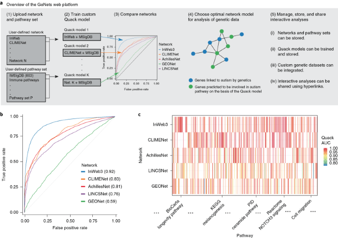
Functional genomics networks are widely used to identify unexpected pathway relationships in large genomic datasets. However, it is challenging to compare the signal-to-noise ratios of

different networks and to identify the optimal network with which to interpret a particular genetic dataset. We present GeNets, a platform in which users can train a machine-learning model

(Quack) to carry out these comparisons and execute, store, and share analyses of genetic and RNA-sequencing datasets.

This work was supported in part by the US National Institutes of Health (NHLBI grants HHSN268201000033C and R01HL096738 to S. Carr; NCI Clinical Proteomics Tumor Analysis Consortium

initiative grant U24CA160034 to S. Carr; grants 1R01MH109903, U01-DK078616, and 5P01HD068250-07 to K.L., A.K., T. Li, and H.H.), the Executive Committee On Research at Massachusetts General

Hospital (Fund for Medical Discovery Award to H.H.), the MGH IRG American Cancer Society (H.H. and K.L.), the Stanley Center at the Broad Institute (grant to K.L., A.K., T. Li, and H.H.),

the Broad Institute (Broadnext10 grant to K.L., A.K., T. Li, and H.H.), the Lundbeck Foundation (Large Thematic Project Grant to K.L., A.K., T. Li, and H.H.), and the Simons Foundation

(SFARI; Research Award to K.L., A.K., T. Li, and H.H.)

Department of Surgery, Massachusetts General Hospital, Boston, MA, USA

Taibo Li, April Kim, Heiko Horn, Liraz Greenfeld & Kasper Lage

Taibo Li, April Kim, Joseph Rosenbluh, Heiko Horn, Liraz Greenfeld, David An, Andrew Zimmer, Arthur Liberzon, Jon Bistline, Ted Natoli, Yang Li, Aviad Tsherniak, Rajiv Narayan, Aravind

Subramanian, Ted Liefeld, Bang Wong, Dawn Thompson, Sarah Calvo, Steve Carr, Jesse Boehm, Jake Jaffe, Jill Mesirov, Nir Hacohen, Aviv Regev & Kasper Lage

Department of Electrical Engineering & Computer Science, MIT, Cambridge, MA, USA

Department of Medical Oncology, Dana-Farber Cancer Institute, Harvard Medical School, Boston, MA, USA

Howard Hughes Medical Institute and Department of Molecular Biology, Massachusetts General Hospital, Boston, MA, USA

Department of Statistics, Harvard University, Cambridge, MA, USA

Department of Medicine, University of California, San Diego, San Diego, CA, USA

Center for Immunology and Inflammatory Diseases, Massachusetts General Hospital, Boston, MA, USA

Department of Surgery, Harvard Medical School, Boston, MA, USA

Howard Hughes Medical Institute, Department of Biology, MIT, Cambridge, MA, USA

Institute for Biological Psychiatry, Mental Health Center Sct. Hans, University of Copenhagen, Roskilde, Denmark

T. Li, A.K., H.H., L.G., D.A., A.Z., J. Bistline, B.W., A.R., and K.L. developed the GeNets platform. T. Li, A.K., J.R., H.H., L.G., D.A., A.Z., A.L., J. Bistline, T.N., Y.L., A.T., R.N.,

A.S., T. Liefeld, B.W., D.T., S. Carr, S. Calvo, J. Boehm, J.J., J.M., N.H., A.R., and K.L. analyzed data and performed experiments. T. Li and K.L. wrote the paper with input from all other

authors. K.L. initiated, designed, and led the project.

Publisher’s note: Springer Nature remains neutral with regard to jurisdictional claims in published maps and institutional affiliations.

a) For a given pathway, we measure its topological properties exemplified here with the 22 genes of the AKT pathway in the InWeb protein-protein interaction network. We make the same

measurements for all genes in the AKT pathway context set (grey squares), in this case 2,449 genes (only 2 of which are shown for illustration) that have at least one connection to an AKT

gene in InWeb. The distributions for 4 of 18 topological properties are shown and illustrate the differences between pathway (dark blue) and context (light grey) distributions. b) This

procedure is repeated for 853 non-redundant pathways in the InWeb network. The distributions of the broader population show that genes in a common pathway have a topological signature that

distinguishes them from context genes. c) Repeating the procedure detailed in b) for the other four networks shows this is a general principle. d) When quantified and compared, it is clear

that each network has a unique distribution of topological metrics [colors as indicated in panels b/c]]. In all panels the x-axis denotes the respective metrics and the y-axis is the

relative frequency (density) of observations. We use the following abbreviations: interaction (int.), member (mbr), distribution (dist.), weighted (Wt.), pathway (P), overall network (N);

e.g. Eigenvector (P) denotes the Eigenvector centrality in the pathway.

Using the 853 pathways, we compute each metric for pathway proteins based on their protein interactions (with other proteins of the same pathway) and individually compute the same metric for

a maximum of 1,500 of the context proteins for each pathway based on how each context protein interacts with the pathway proteins. The x-axis is the metric as indicated (on the log scale to

facilitate visualization) and the y-axis is the scaled density (blue denotes the distribution for pathway members and grey the context genes).

Using the 853 pathways, we compute each metric for pathway genes based on their phylogenetic similarity (with other genes of the same pathway) and individually compute the same metric for a

maximum of 1,500 of the context genes for each pathway based on how each context gene is connected to the pathway genes. The x-axis is the metric as indicated (on the log scale to facilitate

visualization) and the y-axis is the scaled density (orange denotes the distribution for pathway members and grey the context genes).

Using the 853 pathways, we compute each metric for pathway genes based on their correlation in expression (with other genes of the same pathway) and individually compute the same metric for

a maximum of 1,500 of the context genes for each pathway based on how each context gene is correlated to the pathway genes. The x-axis is the metric as indicated (on the log scale to

facilitate visualization) and the y-axis is the scaled density (purple denotes the distribution for pathway members and grey the context genes).

Using the 853 pathways, we compute each metric for pathway genes based on their cell perturbation profiles (with other genes of the same pathway) and individually compute the same metric for

a maximum of 1,500 of the context genes for each pathway based on how each context gene is connected to the pathway genes. The x-axis is the metric as indicated (on the log scale to

facilitate visualization) and the y-axis is the scaled density (green denotes the distribution for pathway members and grey the context genes).

Using the 853 pathways, we compute each metric for pathway genes based on their cancer codependencies (with other genes of the same pathway) and individually compute the same metric for a

maximum of 1,500 of the context genes for each pathway based on how each context gene is codependent to the pathway genes. The x-axis is the metric as indicated (on the log scale to

facilitate visualization) and the y-axis is the scaled density (red denotes the distribution for pathway members and grey the context genes).

Using the 853 pathways, we compute each metric for pathway genes (within each pathway) based on the connections defined by the respective networks. The x-axis is the metric as indicated (on

the log scale to facilitate visualization) and the y-axis is the scaled density (blue: InWeb, red: AchillesNet, green: LINCSNet, purple: GEONet, orange: CLIMENet).

For each functional data set, we thresholded the top positive connections using the original data, network deconvoluted data, and globally silenced data and selected 5 thresholds: 500K (a),

750K (b), 1M (c), 1.25M (d), and 1.5M (e). For each network, method, and threshold, we train and test the performance of Quack using a 70/30 split on the 853 pathways (N = 597 pathways for

training and N = 256 pathways for testing). AUCs are computed based on holdout data and empirical confidence intervals are computed for each of the classifiers by bootstrapping trees from

each forest. Center line, median; error bars, 2.5th and 97.5th percentiles.

For each functional data set, we thresholded the top positive connections using the original data, network deconvoluted data, and globally silenced data and selected 5 thresholds: 500K (a),

750K (b), 1M (c), 1.25M (d), and 1.5M (e). For each network, method, and threshold, we compute the density (# edges / # possible edges) for each of the 853 pathways based on the connections

found in the respective pathways. A null distribution for the density metric is also computed based on N = 250 randomly sampled gene sets of similar size and degree distribution as the

pathway under consideration, from which we compute an empirical p-value for each pathway. The sensitivity is computed by assessing how many of the 853 pathways were deemed significantly

connected at an alpha=0.05 significance level. Center line, median; error bars, 2.5th and 97.5th percentiles.

a) For a given pathway, we measure its topological properties exemplified here with the 21 genes of the AKT pathway in the InWeb protein-protein interaction network. In the matrix, the 18

topological properties are shown as columns and the corresponding values for each of the 21 genes in the AKT pathway (black circles) as rows (metric values correspond to colors as indicated

in the figure legend). One row in this matrix corresponds to one row in the final modeling dataset. We make the same measurements for genes in the context of the AKT pathway (white squares);

only 2 of 2,449 context genes shown in the illustration. b) This procedure is repeated for 853 pathways from which the modeling dataset used to train the classifier is derived. For any

candidate gene in a network, the classifier can assign a probability that it belongs to a pathway (e.g., the AKT pathway) as defined by the candidates’ topological properties in the overall

network and in relation to a specific set of genes (e.g., the 21 AKT genes).

For each network, we score the 30% holdout of 853 pathways (N = 256 pathways) and their context after training and testing the respective classifiers. For each network, we use the classifier

assigned probabilities (assigned to pathways and their contexts) and compute deciles of the predicted probability distribution. Here, the decrease in true positive rate (# of pathway

members / all genes in the decile) in lower deciles further illustrates the predictive power of the classifiers and the consistency between the predicted probability and the true positive

rate. The number of pathway members (N_p) and context genes (N_c) considered in the 30% holdout set for each network are as follows: AchillesNet (N_p = 1,323; N_c = 202,532), GEONet (N_p =

3,676; N_c = 240,465), InWeb (N_p =6,584; N_c = 220,077), CLIMENet (N_p =1,482; N_c = 141,998), LINCSNet (N_p =2,279; N_c =227,554).

a) From the 31 candidate genes discovered in Main Text Fig. 2d, de annotated genes in genome-wide significant schizophrenia loci with orange and genes in which de novo mutations have been

found in neurodevelopmental delay with purple. b) Genes under brain-specific regulation are also annotated (large nodes correspond to genes that have brain-specific eQTLs). Network layouts

are identical in panels a, b and Main Text Fig. 2d allowing gene names to be inferred.

By permuting the values of each topological metric being evaluated it is possible to estimate the overall importance of each topological metric across networks. Here the topological

properties are in descending order by their average rank across networks. The y-axis is the rank (1-18), where 18 is most important metric for distinguishing pathway members and 1 is least

important. We use the following abbreviations weighted (Wt.), pathway (P), overall network (N) and local clustering coefficient (LCC), so that LCC (P) and LLC (N) means local clustering

coefficient in the pathway and network, respectively. Closeness and Eigenvector centrality is consistently important across networks (column 18 and 17, respectively), while there is

significant variation in the predictive power of e.g., the local clustering coefficient in the network [LCC (N), column 8]. We also observe that some metrics such as the degree in the

pathway (column 1), are less important in all networks when controlling for others topological metrics.

We plotted the network-specific eigenvector centralities of genes in the PDGF pathway (n = 121 genes), ERBB1 downstream pathway (n = 105 genes), and E2F pathway (n = 74 genes), indicated by

row. Large nodes denote high values and small nodes denote low values with respect to a specific pathway across networks. Only pathway members that have network information in one of the

networks are shown. To enable a straightforward visual comparison, we pooled all five networks and laid out the genes in each pathway based on this one meta-network. Edges connecting genes

in a given pathway correspond to the network indicated by the column. Although non-pathway genes have been omitted for clarity, the pathways are embedded in very complex network-specific

neighborhoods involving thousands (ranging from 1,386 to 4,208) of context genes. While the eigenvector centrality is generally high for pathway members across all networks, we also observe

considerable divergence in the gene-specific patterns and strengths of these values, and in the patterns of connections between pathway sets.

a) For each of N = 45 neural pathways presented in Main Text Fig. 2a, we randomly masked 30% of pathway genes and asked each of Quack, SANTA, and GeneMANIA to distinguish holdout genes based

on their relationship with the 70% seed genes. We used InWeb for Quack and SANTA, and default network for GeneMANIA. AUCs were calculated based on method-specific scores and pathway

membership, and plotted as distributions for each method. b) For each of the N = 853 canonical MSigDB pathways presented in Main Text Fig. 1c, we repeated the same analyses for Quack and

SANTA and plotted AUC distributions. Center line, median; box limits, upper and lower quartiles; whiskers, 1.5x interquartile range; points, outliers.

Supplementary Figures 1–15, Supplementary Tables 1 and 2 and Supplementary Notes 1–8

853 curated canonical pathways from the Molecular Signatures Database

Anyone you share the following link with will be able to read this content: