Nonreciprocal nonlinear responses in moving charge density waves

ABSTRACT The incommensurate charge density wave states (CDWs) can exhibit steady motion in the flow limit after depinning, behaving as a nonequilibrium system with time-dependent states.

Since the moving CDW, like an electric current, breaks both time-reversal and inversion symmetries, one may speculate the emergence of nonreciprocal nonlinear responses from such motion.

However, the moving CDW order parameter is intrinsically time-dependent in the lab frame, and it is known to be challenging to evaluate the responses of such a time-varying system. In this

work, following the principle of Galilean relativity, we resolve this time-dependent hard problem in the lab frame by mapping the system to the comoving frame with static CDW states through

the Galilean transformation. We explicitly show that the nonreciprocal nonlinear responses would be generated by the movement of CDW states through violating Galilean relativity. SIMILAR

CONTENT BEING VIEWED BY OTHERS SCHRÖDINGER–POISSON SYSTEMS UNDER GRADIENT FIELDS Article Open access 20 September 2022 OBSERVATION OF OPTICAL DE BROGLIE–MACKINNON WAVE PACKETS Article 19

January 2023 GENERALISING QUANTUM IMAGINARY TIME EVOLUTION TO SOLVE LINEAR PARTIAL DIFFERENTIAL EQUATIONS Article Open access 30 August 2024 INTRODUCTION Nonreciprocal nonlinear responses

can manifest when inversion symmetry (and time-reversal symmetry in many cases) is broken1,2. These phenomena have garnered significant theoretical and experimental attention in recent

years, notably in phenomena such as nonlinear Hall effects3,4 and nonreciprocal superconducting effects2,5,6,7. However, while much focus has been near the equilibrium states, nonreciprocal

nonlinear responses in nonequilibrium systems with time-dependent states remain largely unexplored. Theoretical investigation of such responses in nonequilibrium states is challenging due to

the inherent time dependence and dynamic nature of these systems. In condensed matter physics, current-driven systems can exhibit nonequilibrium behavior and intrinsic time-dependence. For

example, certain symmetry-breaking orders would undergo motion once they surpass impurity-pinning effects under an electric field beyond the threshold. A notable example is the

incommensurate charge density wave (CDW), where intriguing dynamical properties emerge upon depinning8,9,10,11,12. In the limit of large current, these CDW states flow steadily, representing

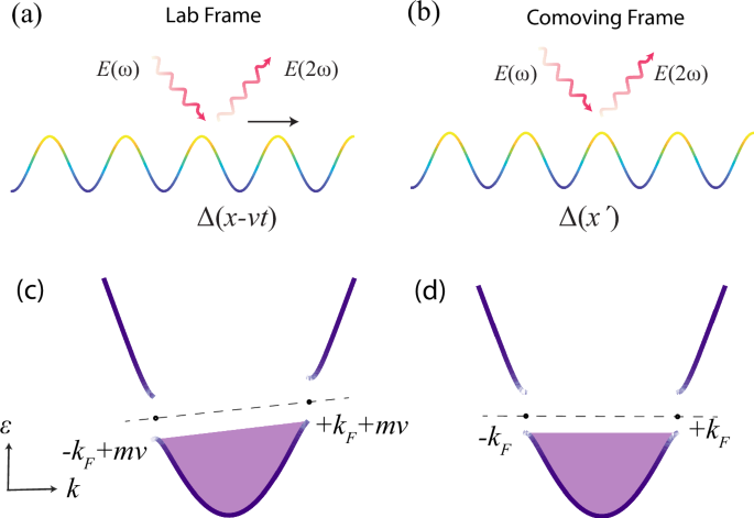
a nonequilibrium steady state. A CDW motion breaks both inversion and time-reversal symmetries (see illustrations in Fig. 1a, c), as implied in the seminar work by Allender, Bray, and

Bardeen13. One may naturally ask whether there are any finite nonreciprocal nonlinear responses induced by the current-driven motion (Fig. 1a). However, directly addressing this problem is

challenging due to the intrinsic time dependence of a moving CDW in the lab frame. On the other hand, in classical physics, we know that the principle of relativity is often powerful in

simplifying a problem by changing inertial frames. Following this principle, the moving CDW problem can be reconsidered in the comoving frame, where the CDW state becomes static. In contrast

to the lab frame, the asymmetry induced by the external current appears to vanish in the comoving frame as illustrated in Fig. 1b, d. As a result, one may expect that nonreciprocal

nonlinear responses vanish in the comoving frame. Looking at the nonreciprocal nonlinear responses for moving states within both the lab and comoving frame is indeed puzzling. Motivated by

exploring nonreciprocal nonlinear responses in nonequilibrium systems with time-dependent state and the aforementioned puzzle, we explicitly study nonreciprocal nonlinear responses in moving

CDW states in this work. We begin with a simple one-dimensional (1D) CDW model, where the CDW order parameter moves spatially at a constant velocity. Using the field theory approach, we

identify that the moving CDW state can be mapped to a static one through the Galilean transformation. The transformation is identical to the change of inertial frames from the lab frame to

the comoving frame with the CDW. We also argue that the Galilean transformation dictates the invariance of the optical conductivity in the lab and comoving frames, facilitating the

straightforward solution of optical responses in the comoving frame. Based on this understanding, we show that the nonreciprocal nonlinear responses are absent with Galilean relativity,

where the single-particle dispersion is simply quadratic and thus Galilean invariant. By introducing a quartic term to violate Galilean relativity, we explicitly show that nonreciprocal

nonlinear responses would appear. RESULTS A MOVING CDW MODEL AND GALILEAN TRANSFORMATION Let us first illustrate how we can map a time-dependent problem in the lab frame onto a

time-independent problem in the comoving using the principle of relativity. We start with the simplest 1D continuum model with a moving CDW, which has been widely used to study the dynamics

of a CDW12,13,14: $${\mathcal{L}}=i{\psi }^{\dagger }{\partial }_{t}\psi -\frac{1}{2m}{\partial }_{x}{\psi }^{\dagger }{\partial }_{x}\psi -{\psi }^{\dagger }V(x-vt)\psi ,$$ (1) where

\({\mathcal{L}}\) is the Lagrangian, ∂_x_ denotes \(\frac{\partial }{\partial x}\), _ψ_(_x_, _t_) is a field operator for electrons, _m_ is an effective mass, and we set _ℏ_ = 1 in the main

text. The CDW order parameter is $$V(x-vt)=2\Delta \cos (2{k}_{F}(x-vt))$$ (2) with _v_ the drift velocity of the CDW. The wave vector of the CDW is denoted as 2_k__F_, where

\({k}_{F}=\sqrt{2m{\epsilon }_{F}}\) is the Fermi wave vector at the Fermi energy _ϵ__F_. The electronic energy dispersion acquires an energy gap _Δ_ at the Fermi level, corresponding to the

CDW order parameter. Such CDW states emerge in quasi-1D systems12. The Lagrangian density \({\mathcal{L}}\) describes the dynamics of quasi-1D CDW states driven by an electric current in

the flow region12,13,14. We shall assume disorder effects are negligible in the flow region. Note that due to the lack of dissipations induced by the disorder effects, a finite electric

field infinitely accelerates electrons. Instead, what drives the moving CDW state is the DC electric current other than the electric field. In this case, the electric current arises from the

time-varying of the CDW phase12. To eliminate the time dependence of the CDW order parameter, we introduce the comoving frame by performing the Galilean transformation on the coordinates

\({x}^{{\prime} }=x-vt,{t}^{{\prime} }=t\), \({\partial }_{t}={\partial }_{t}^{{\prime} }-v{\partial }_{{x}^{{\prime} }}\), \({\partial }_{x}={\partial }_{{x}^{{\prime} }}\). The field

operator transforms as \(\psi ={e}^{i\eta (x,t)}{\psi }^{{\prime} }\) with the phase factor \(\eta (x,t)=mvx-\frac{1}{2}m{v}^{2}t\); see Method section for details. After this

transformation, the Lagrangian in the moving frame reads $${{\mathcal{L}}}^{{\prime} }=i{\psi }^{{\prime} \dagger }{\partial }_{{t}^{{\prime} }}{\psi }^{{\prime} }-\frac{1}{2m}{\partial

}_{{x}^{{\prime} }}{\psi }^{{\prime} \dagger }{\partial }_{{x}^{{\prime} }}{\psi }^{{\prime} }-{\psi }^{{\prime} \dagger }V({x}^{{\prime} }){\psi }^{{\prime} }$$ (3) with \(V({x}^{{\prime}

})=2\Delta \cos (2{k}_{F}{x}^{{\prime} })\). Comparing Eq. (1) with Eq. (3), we can see that the exact Galilean invariance does not exist due to the CDW order parameter. However, the problem

in the lab frame with the moving potential _V_(_x_ − _v__t_) is mapped to the one in the comoving frame with the static potential \(V({x}^{{\prime} })\). As there are no extra new terms

after Galilean transformation, we would call the system exhibits _Galilean relativity_ in this case. Because of this Galilean relativity, the nonlinear responses would not appear since the

energy dispersion is simply quadratic in the comoving frame without time dependence. In general, there is no exact Galilean relativity in solids. In this work, we invoke a violation of

Galilean relativity by introducing a quartic term: $$\delta {\mathcal{L}}=-\lambda {\partial }_{x}^{2}{\psi }^{\dagger }{\partial }_{x}^{2}\psi ,$$ (4) which is allowed by any symmetries. In

this case, the total Lagrangian is \({{\mathcal{L}}}_{t}={\mathcal{L}}+\delta {\mathcal{L}}\). After the Galilean transformation, it is straightforward to show the Lagrangian in the

comoving frame becomes \({{\mathcal{L}}}_{t}^{{\prime} }={{\mathcal{L}}}^{{\prime} }+\delta {{\mathcal{L}}}^{{\prime} }\), where \(\delta {{\mathcal{L}}}^{{\prime} }\) represents the quartic

term in the comoving frame: $$\begin{array}{lll}\delta {{\mathcal{L}}}^{{\prime} }=-\lambda {\psi }^{{\prime} \dagger }{\partial }_{{x}^{{\prime} }}^{4}{\psi }^{{\prime} }-\lambda

{m}^{4}{v}^{4}{\psi }^{{\prime} \dagger }{\psi }^{{\prime} }+4i\lambda {m}^{3}{v}^{3}{\psi }^{{\prime} \dagger }{\partial }_{{x}^{{\prime} }}{\psi }^{{\prime} }\\ \quad\qquad+\,6\lambda

{m}^{2}{v}^{2}{\psi }^{{\prime} \dagger }{\partial }_{{x}^{{\prime} }}^{2}{\psi }^{{\prime} }-4i\lambda mv{\psi }^{{\prime} \dagger }{\partial }_{{x}^{{\prime} }}^{3}{\psi }^{{\prime}

}.\end{array}$$ (5) It can be seen that when we consider a more general dispersion, beyond the simplistic quadratic band, residual terms emerge in the Lagrangian, which cannot be eliminated

in the comoving frame. It is also interesting to note that the terms that are odd in momentum in Eq. (5) break inversion and time-reversal symmetries, which is expected for moving CDWs but

forbidden by Galilean relativity previously. As we will see later, the cubic-momentum term, i.e., the last term in Eq. (5), results in nonreciprocal nonlinear responses. It is worth noting

that we can map the Lagrangian to be time-independent for the moving CDW model even with the quartic term via Galilean transformation. This allows us to evaluate some interesting effects

that previously were hard to demonstrate in a time-dependent system. To be specific, we shall focus on the nonreciprocal nonlinear responses next. THE INVARIANCE OF FINITE FREQUENCY

RESPONSES UNDER GALILEAN TRANSFORMATION We next show that the nonreciprocal nonlinear responses can be equivalently calculated in the comoving frame. The conductivity of nonlinear responses

is defined by expanding the current density in the powers of external fields. For example, the _n_-th order harmonic generation in the lab frame is obtained from \({J}_{x}(n\omega )={\sigma

}_{xx}(n\omega ){E}_{x}^{n}(\omega )\), where _n_ is a positive integer and _ω_ is the incident photon energy (_ℏ_ = 1), _E__x_ denotes the electric field along _x_-direction. Note that we

have simplified subscript in the conductivity; for example, the second-order conductivity tensor _σ__x__x__x_(2_ω_) would be simply labeled with _σ__x__x_(2_ω_) or _σ_(2_ω_) below. Now we

show how the optical conductivity transforms upon a Galilean transformation by using the Galilean transformation relation of the electric field and current. According to the minimal coupling

principle, an electromagnetic field would appear in the Lagrangian by replacing the ∂_i__ψ_ in Eq. (1) as (∂_i_ + _i__e__A__i_)_ψ_, ∂_i__ψ_† as (∂_i_ − _i__e__A__i_)_ψ_†15. Then the

current-density operator is \({j}_{x}=\frac{\partial {{\mathcal{L}}}_{t}}{\partial {A}_{x}}{| }_{{A}_{x} = 0}\). Upon the Galilean transformation \(\psi ={e}^{i\eta (x,t)}{\psi }^{{\prime}

}\), we find that the current-density operators in the lab and comoving frames satisfy $${\hat{j}}_{x}{\scriptstyle{\!\!\!\prime}\atop}={\hat{j}}_{x}+ev{\psi }^{{\prime} \dagger }{\psi

}^{{\prime} },$$ (6) where \({\hat{j}}_{x}{\scriptstyle{\!\!\!\prime}\atop}\) is the current operator deduced from the Lagrangian \({{\mathcal{L}}}_{t}^{{\prime} }\). See the explicit

derivations in Supplementary Note 2. Note that Eq. (6) holds even with the quartic term. Sandwiching the current operator with the ground state, we obtain the well-known Galilean

transformation for the current $${J}_{x}^{{\prime} }(t)={J}_{x}(t)+evN,$$ (7) where \({t}^{{\prime} }=t\) is used and the total electron number \(N=\int\,d{x}^{{\prime} }\langle {\psi

}^{{\prime} \dagger }{\psi }^{{\prime} }\rangle\), where 〈〉 denotes the average over the ground states. The form of Eq. (7) is consistent with the one obtained from the relativity theory in

classical electrodynamics (Supplementary Note 1). Moreover, as shown in Supplementary Note 2B, we argue that Eq. (7) holds for a generic energy dispersion by performing Galilean

transformation in the momentum space, where the group velocity of each electron is uniformly shifted by _v_. Operating ∫ _d__t__e_−_i__n__ω__t_ on both sides, we find \({J}_{x}^{{\prime}

}(n\omega )={J}_{x}(n\omega )\) for _ω_ ≠ 0. Here we consider a finite frequency response because the DC conductivity with _ω_ = 0 is divergent without dissipations. Note that the current

_e__v__N_ in Eq. (7) does not contribute to the finite frequency response as _N_ is time-independent due to the conservation of total electron number in the system. On the other hand, the

electric fields of light in the two frames are the same \({{\boldsymbol{E}}}^{{\prime} }={\boldsymbol{E}}\) when there are no external magnetic fields16 and Supplementary Note 1, resulting

in \({E}_{x}(n\omega )={E}_{x}^{{\prime} }(n\omega )\). Using \({\sigma }_{xx}^{{\prime} }(n\omega )={J}_{x}^{{\prime} }(n\omega )/{E}_{x}^{{\prime} n}(\omega )\), we find that the optical

conductivity in the lab frame and comoving frame are equal: $${\sigma }_{xx}(n\omega )={\sigma }_{xx}^{{\prime} }(n\omega ).$$ (8) Hence, the finite frequency conductivity in the lab frame

and in the comoving frame related by a Galilean transformation are equal. For the simplest case, there is no quartic term (_λ_ = 0), so that the system exhibits Galilean relativity. In this

case, there is no inversion symmetry breaking in the comoving frame even with a moving CDW state. As a result, there are no nonreciprocal nonlinear responses. The _k_2 dispersion is indeed

special. In the Method section, we also discuss how the nonlinear transport response can be allowed when the quartic term is further added. THE NONRECIPROCAL NONLINEAR RESPONSES IN THE

MOVING CDW STATES Now we are ready to unveil the non-reciprocal nonlinear responses within an intrinsic time-dependent system: the moving CDW states described by the Lagrangian

\({{\mathcal{L}}}_{t}\). As demonstrated earlier, the finite frequency conductivity remains unchanged under the Galilean transformation. Consequently, we can address this challenging problem

in the comoving frame using the Lagrangian \({{\mathcal{L}}}_{t}^{{\prime} }\) To calculate the nonreciprocal nonlinear responses, we first deduce the low-energy Hamiltonian given by

\({{\mathcal{L}}}_{t}^{{\prime} }\). According to Eq. (5) and using \({\psi }_{{k}_{x}^{{\prime} }}^{{\prime} }=\int\,d{x}^{{\prime} }{e}^{-i{k}_{x}^{{\prime} }x}{\psi }^{{\prime}

}({x}^{{\prime} })\), the energy dispersion in the comoving frame becomes $${\epsilon }_{{k}_{x}^{{\prime} }}=\frac{{k}_{x}^{{\prime} 2}}{2m}+4\lambda {m}^{3}{v}^{3}{k}_{x}^{{\prime}

}+6\lambda {m}^{2}{v}^{2}{k}_{x}^{{\prime} 2}+4\lambda mv{k}_{x}^{{\prime} 3}+\lambda {k}_{x}^{{\prime} 4}.$$ (9) Then we can expand the momentum of the states near the Fermi momentum

(\({k}_{x}^{{\prime} }={\tilde{k}}_{x}+s{k}_{F}\) with _s_ = ± branch) and consider the CDWs would couple these two branches. The resulting low-energy Hamiltonian (up to the second order in

\({\tilde{k}}_{x}\)) in the comoving frame is given by $${H}_{0}({\tilde{k}}_{x})=\left(\begin{array}{cc}{\tilde{\epsilon }}_{+,{\tilde{k}}_{x}}&\Delta \\ \Delta &{\tilde{\epsilon

}}_{-,{\tilde{k}}_{x}}\end{array}\right)$$ (10) where $${\tilde{\epsilon }}_{s,{\tilde{k}}_{x}}=(s{\tilde{v}}_{F}+\delta {v}_{F}){\tilde{k}}_{x}+(s\tilde{\beta }+\delta \beta

){\tilde{k}}_{x}^{2}+s\tilde{\alpha },$$ (11) Here, the coefficients are \({\tilde{v}}_{F}={v}_{F}+12\lambda {m}^{2}{v}^{2}{k}_{F}+4\lambda {k}_{F}^{3},\delta {v}_{F}=4\lambda

{m}^{3}{v}^{3}+12\lambda mv{k}_{F}^{2},\delta \beta =\frac{1}{2m}+6\lambda {m}^{2}{v}^{2}+6\lambda {k}_{F}^{2},\tilde{\alpha }=4\lambda mv{k}_{F}({k}_{F}^{2}+{m}^{2}{v}^{2}),\tilde{\beta

}=12\lambda mv{k}_{F}\). Importantly, when _λ_ ≠ 0, the \(s\tilde{\beta }{\tilde{k}}_{x}^{2}\) term that breaks the inversion symmetry is finite, which would be essential for the

second-order nonlinear optical responses as we would show next. Inserting the Hamiltonian \({H}_{0}({\tilde{k}}_{x})\) into the formula of nonlinear optical responses17 (see the Method

section and Supplementary Note 4 for details), we find that the second-order nonlinear optical conductivity is given by $${\sigma }^{(2)}(2\omega )=\frac{\tilde{\beta }{e}^{3}}{2{\omega

}^{2}}\left[2F\left(\frac{\omega +i\gamma }{\Delta }\right)+F\left(\frac{2\omega +i\gamma }{\Delta }\right)\right].$$ (12) Here, _ω_ is the photon frequency, the function

\(F(a)=\frac{1}{2\pi }[\frac{\pi }{a}+\frac{8}{a\sqrt{{a}^{2}-4}}(\,\text{arctanh}(\frac{a}{\sqrt{{a}^{2}-4}})-\text{arctanh}\,(\frac{a-2}{\sqrt{{a}^{2}-4}}))]\), and \(F(\frac{\omega

+i\gamma }{\Delta })\), \(F(\frac{2\omega +i\gamma }{\Delta })\) arise from one-photon and two-photon processes, respectively. The one-photon and two-photon exhibit a leading scaling of

(_ω_−2_Δ_)−1/2 and (_ω_−_Δ_)−1/2, respectively. A typical scaling for photoconductivity in 1D limit. Note that _γ_ is a small damping parameter, which is related to the lifetime of an

excited electron and can be finite even in a clean system. The imaginary part of _σ_(2_ω_) representing the second harmonic absorption is plotted in Fig. 2. Note that the real part of

_σ_(2_ω_) is directly related to Im[_σ_(2_ω_)] according to the Kramers–Kronig relations18. The one-photon and two-photon absorption peaks near _ω_ = 2_Δ_ and _ω_ = _Δ_ can be clearly seen.

It is worth noting that \(\sigma (2\omega )\propto \tilde{\beta }\propto \lambda mv\), while \(\tilde{\beta }\) arises from the cubic term in Eq. (9) induced by the additional quartic term

in the lab frame. Moreover, as expected, the second-order nonreciprocal nonlinear responses are finite only when the CDW states are moving, i.e., _v_ ≠ 0 so that \(\tilde{\beta }\,\ne\, 0\).

Therefore, we have explicitly demonstrated the nonreciprocal nonlinear responses in the moving CDW states through the Galilean transformation. DISCUSSION It is important to note that with

an external excitation at optical frequencies above the CDW energy gap, the quasi-particle effects that we have discussed are dominant. It should be distinguished from the transport region,

where the interaction between impurities and collective modes of the CDW should dominate finite frequency responses11,12. As shown in Fig. 3a, in general, the current-driven CDW states

exhibit three distinct regions: the pinned, creep, and flow regions according to the strength of the electric field. The pinned region may exhibit nonlinear responses due to the distortion

of the CDW, while the nonlinear responses are expected to peak around the creep region where the depinning motion of CDW is strongest. Our speculation for the nonlinear responses in the

transport region (_ω_ ≪ _Δ_) is shown in Fig. 3b, where the nonlinear responses mostly stem from the creep motion of the sliding density wave. In the optical limit (_ω_ ~ _Δ_), the

quasiparticle effects would be more crucial, which fits our interest in this work. In this case, our results imply that the second-order nonlinear conductivity within the flow region

linearly increases with the current in the case without emergent Galilean relativity [see the solid blue lines in Fig. 3c]. We next discuss the some approximations we have made in our moving

CDW model in the main text. First, the continuum model approximation is used in capturing the energy dispersion. We expect that the continuum model approximation is valid when the CDW gap

is far away from the Brillouin zone boundary (or much smaller than the bandwidth) so that the lattice periodic potential is not crucial. Near the Brillouin zone boundary, the underlying

periodic lattice potential would become crucial and open the gap in energy dispersion. Second, we have assumed the disorder effects can be negligible in the flow region. When the Galilean

transformation is performed, the presence of disorder potential in the lab frame would result in moving disorders in the comoving frame. However, the CDW order has gapped out the states so

that the moving disorders do not have states to scatter near Fermi energy. As a result, we expect that our results based on Galilean transformation would not be affected by the presence of

weak disorder effects as long as the speed of moving disorders is not large enough to overcome the CDW gap. The current-driven CDW states in the flow region behave as nonequilibrium steady

states in this work, which breaks time-reversal and inversion symmetry. We would like to emphasize here that the current carried by the moved CDW state arises from the time-dependent CDW

phase change in real space12, which resembles the phase gradient-induced current in superconductors. It should be distinguished from the single-particle currents driven by DC fields in

metals. In other words, what is applied externally is the current instead of the DC electric fields for the moving CDW. In practice, due to thermal effects or other dissipations, some small

DC electric field may be built in the flow region. The DC fields can directly couple with the electrons. In insulators, the presence of electric fields can result in the Landau–Zener

tunneling19. However, as we estimated in the Supplementary Note 5, the Landau–Zener tunneling probability is negligible for the moving CDW state. Our analysis in the main text thus would not

affected by the presence of small DC electric fields with negligible Landau–Zener tunneling effects. In the main text, our model is analyzed in the 1D limit. In practice, the system can

exhibit a higher dimension. Here, we briefly discuss the 2D limit by introducing the momentum _k__y_. In this case, the normal-state dispersion can be described by the Hamiltonian (in the

lab frame): \(H({\boldsymbol{k}})=\frac{{k}_{x}^{2}}{2m}+\lambda {k}_{x}^{4}-\mu ({k}_{y})\), where \(\mu ({k}_{y})=\mu +(2{t}_{\perp }\cos {k}_{y}-2{t}_{\perp })\), and _t_⊥ is the hopping

parameter along the _y_-direction. In this form, the 2D system can be regarded as a set of 1D subbands labeled by _k__y_, with the chemical potential shifted by \((2{t}_{\perp }\cos

{k}_{y}-2{t}_{\perp })\). When 4_t_⊥ < _Δ_, the system is expected to remain gapped and behave as quasi-1D. For each _k__y_, the Fermi energy lies within the gap, allowing the system to

be treated as a 1D problem. In general, the gap can also exhibit _k__y_ dependence as well. As a result, the inverse square-root singularity would be broadened by _k__y_ integral in Fig. 3.

On the other hand, in the limit of large hopping (4_t_⊥ > _Δ_), the energy shift due to hopping along the _y_-direction can overcome the CDW gap, making the system metallic. In this case,

the situation becomes more complex, as the presence of low-energy electrons at the Fermi level allows scattering with impurities. As a result, the current would primarily be carried by free

electrons rather than the moving CDW. Unfortunately, this scenario is beyond our theoretical consideration. In summary, we have demonstrated the nonreciprocal nonlinear responses in a

nonequilibrium system with time-dependent states—moving CDW states through Galilean transformation. It is important to note that moving CDW states are non-perturbative nonequilibrium steady

states. As a result, our analysis is in sharp contrast with the conventional perturbative calculations of non-linear responses in the lab frame. Looking ahead, we encourage experimentalists

to revisit the quasi-1D CDW materials such as TaS3, NbSe3, etc.12, and explore their nonreciprocal nonlinear optical responses above the gap using advanced terahertz light measurements. A

comparative analysis of experimental results with our theoretical insights would be intriguing. Furthermore, we note that the nonreciprocal nonlinear responses would also appear in some

other current-driven systems, such as superconductors20,21,22, Weyl materials23. However, it is worth pointing out that there is no clear intrinsic time dependence in the lab frame for these

systems, which is in contrast with the moving CDW states. Nevertheless, it would be interesting to revisit the nonlinear nonreciprocal responses in current-driven superconductors or

topological materials in the comoving frame with our theoretical framework. One challenge is that our analysis in this work starts from simple models, which may be difficult to apply

materials with complicated low-energy dispersions. However, in some materials, the low-energy dispersion can be described with a simple Hamiltonian. In this case, our theoretical framework

based on Galilean transformations can be carried out and offer insights into the external electromagnetic field responses in the nonequilibrium region. METHODS GALILEAN TRANSFORMATION ON THE

FIELD OPERATOR The simplest Lagrangian we are dealing with in this work carries the following form: $${\mathcal{L}}=i{\psi }^{\dagger }{\partial }_{t}\psi -\frac{1}{2m}{\partial }_{i}{\psi

}^{\dagger }{\partial }_{i}\psi -{\psi }^{\dagger }V(x,t)\psi .$$ (13) Let us perform the Galilean transformation: \({x}^{{\prime} }=x-vt\), \({t}^{{\prime} }=t\), \(\frac{\partial

}{\partial t}=\frac{\partial }{\partial {t}^{{\prime} }}+\frac{\partial {x}^{{\prime} }}{\partial t}\frac{\partial }{\partial {x}^{{\prime} }}=\frac{\partial }{\partial {t}^{{\prime}

}}-v\frac{\partial }{\partial {x}^{{\prime} }}\), \(\frac{\partial }{\partial x}=\frac{\partial }{\partial {x}^{{\prime} }}\). To compensate for the coordinate changes, the field operator

should also been transformed $$\psi ={e}^{i\eta ({x}^{{\prime} },{t}^{{\prime} })}{\psi }^{{\prime} }.$$ (14) After the transformation, the Lagrangian becomes

$$\begin{array}{lll}{{\mathcal{L}}}^{{\prime} }=i{\psi }^{{\prime} \dagger }{\partial }_{{t}^{{\prime} }}{\psi }^{{\prime} }-\left[{\partial }_{{t}^{{\prime} }}\eta -v{\partial

}_{{x}^{{\prime} }}\eta +\frac{1}{2m}{({\partial }_{{x}^{{\prime} }}\eta )}^{2}\right]{\psi }^{{\prime} \dagger }{\psi }^{{\prime} }\\\,\qquad -iv{\psi }^{{\prime} \dagger }{\partial

}_{{x}^{{\prime} }}{\psi }^{{\prime} }-\frac{i}{2m}({\partial }_{{x}^{{\prime} }}\eta )\left[\left({\partial }_{{x}^{{\prime} }}{\psi }^{\dagger }\right){\psi }^{{\prime} }-{\psi }^{\dagger

}{\partial }_{{x}^{{\prime} }}\psi \right]\\ \,\qquad-\frac{1}{2m}{\partial }_{{x}^{{\prime} }}{\psi }^{{\prime} \dagger }{\partial }_{{x}^{{\prime} }}{\psi }^{{\prime} }-{\psi }^{{\prime}

\dagger }{V}^{{\prime} }({x}^{{\prime} },{t}^{{\prime} }){\psi }^{{\prime} }.\end{array}$$ (15) To cancel the term in \({\psi }^{{\prime} \dagger }{\partial }_{{x}^{{\prime} }}{\psi

}^{{\prime} }\), $$-iv+\frac{i}{m}{\partial }_{{x}^{{\prime} }}\eta =0.$$ (16) Then it requires $${\partial }_{{x}^{{\prime} }}\eta =mv$$ (17) We can further fix the form of _η_ by

considering the system is Galilean invariant in the case without spatial dependent potential \({V}^{{\prime} }({x}^{{\prime} },{t}^{{\prime} })=V(x,t)=0\). In this case, the Lagrangian would

exhibit the same form in the lab frame and moving frame if $${\partial }_{{t}^{{\prime} }}\eta -v{\partial }_{{x}^{{\prime} }}\eta +\frac{1}{2m}{({\partial }_{{x}^{{\prime} }}\eta

)}^{2}=0.$$ (18) Now we obtain the phase factor on the field operator under Galilean transformation is given by $$\eta =mv{x}^{{\prime} }+\frac{1}{2}m{v}^{2}{t}^{{\prime}

}=mvx-\frac{1}{2}m{v}^{2}t.$$ (19) In the case of moving CDW, the potential _V_(_x_, _t_) = _V_(_x_ − _v__t_) is mapped to \(V({x}^{{\prime} })\) in the comoving frame after the Galilean

transformation. NONLINEAR TRANSPORT INDUCED BY THE DISPERSION WITHOUT GALILEAN RELATIVITY To further highlight that the _k_2 dispersion is special, we now show the nonlinear transport for

the energy dispersion \({\epsilon }_{{k}_{x}}=\frac{{k}_{x}^{2}}{2m}+\lambda {k}_{x}^{4}\) in the absent of the CDW order parameter. We shall consider a DC plus a small AC component of the

electric current: \(J(t)={J}_{0}+{J}_{ac}\cos (\omega t)\). The DC component is to break the inversion symmetry. It would be expected that the cubic nonlinear responses _V_3 = _R_3_J_3 (_V_3

is the voltage, _R_3 is the resistance) would give rise to a 2_ω_-signal: \({V}_{2\omega }=3{R}_{3}{J}_{0}{J}_{ac}^{2}\). For the moment, we consider the electronic system without CDW but

with finite relaxation. From the Boltzmann transport equation (see Supplementary Note 3), we can derive that the 2_ω_-component of conductivity given by the third-order nonlinear response is

$${\sigma }^{(3)}(2\omega )=\frac{{e}^{4}\Gamma (\omega ,\tau )}{4}\int\,\frac{d{k}_{x}}{2\pi }{f}^{(0)}{\partial }_{{k}_{x}}^{3}v({k}_{x})=6{e}^{4}\lambda n\Gamma (\omega ,\tau ),$$ (20)

where the factor \(\Gamma (\omega ,\tau )=\frac{1}{{(2i\omega +{\tau }^{-1})}^{2}(i\omega +{\tau }^{-1})}+\frac{\tau }{(2i\omega +{\tau }^{-1})(i\omega +{\tau }^{-1})}+\frac{1}{(2i\omega

+{\tau }^{-1}){(i\omega +{\tau }^{-1})}^{2}}\), _τ_ is the scattering time, _f_(0) is the Fermi distribution function, the electron velocity \(v({k}_{x})=\frac{\partial \epsilon

({k}_{x})}{\partial {k}_{x}}\), and the electron density \(n=\int\,\frac{d{k}_{x}}{2\pi }{f}^{(0)}(\epsilon ({k}_{x})-{\epsilon }_{F})\). From the Eq. (20), it can be seen that the

nonreciprocal nonlinear responses giving _σ_(2_ω_) signal are absent in the simplest quadratic band dispersion (_λ_ = 0). It becomes finite when the quartic term is introduced. In the main

text, we have also obtained the optical second harmonic generation optical conductivity _σ_(2_ω_), i.e., Eq. (12). Now let us compare the magnitude between these two nonlinear conductivity.

It can be seen that $$\frac{{\sigma }^{(2)}(2\omega )}{{\sigma }^{(3)}(2{\omega }^{{\prime} })E} \sim \frac{\frac{\tilde{\beta }{e}^{3}}{2{\omega }^{2}}}{6{e}^{4}\lambda n\Gamma ({\omega

}^{{\prime} },\tau )E}$$ (21) Here _ω_ is photon frequency and \({\omega }^{{\prime} }\) is the transport frequency. The numerator only refers to the imaginary part of _σ_(2)(2_ω_) here.

Although there are peaks around _ω_ = _Δ_ and 2_Δ_, _σ_(2)(2_ω_) are at order of \(\frac{\tilde{\beta }{e}^{3}}{2{\omega }^{2}}\) (see Fig. 3). Note that the electric field _E_ that drives

the DC current _J_0 appears on the denominator to fix the dimension. In the optical limit (\({\omega }^{{\prime} }\gg {\tau }^{-1}\)), \(\Gamma ({\omega }^{{\prime} },\tau ) \sim

\frac{1}{{\omega }^{{\prime} 3}}\). Inserting \(\tilde{\beta }=12mv{k}_{F}\), _m__v__F_ = _π__n_, we estimated $$\frac{{\sigma }^{(2)}(2\omega )}{{\sigma }^{(3)}(2{\omega }^{{\prime} })E}

\sim \frac{{\omega }^{{\prime} 3}}{{\omega }^{2}\Delta }\frac{v}{{v}_{F}}\frac{\pi \Delta }{eE{k}_{F}^{-1}}.$$ (22) Note that \({k}_{F}^{-1} \sim a\), where _a_ is the lattice constant.

Using some reasonable parameters: the CDW moving velocity _v_ ~ 100 m/s, the Fermi velocity _v__F_ ~ 106 m/s, CDW gap _Δ_ ~ 0.1 eV, the lattice constant _a_ = 3 × 10−10 m, and the electric

field _E_ = 105 V/mm, we expect $$\frac{{\sigma }^{(2)}(2\omega )}{{\sigma }^{(3)}(2{\omega }^{{\prime} })E} \sim \frac{{\omega }^{{\prime} 3}}{{\omega }^{2}\Delta }.$$ (23) Therefore, the

relative magnitude of these two nonlinear responses is mostly determined by their frequency. However, it should be noted that these two scenarios are distinct measurements. OPTICAL RESPONSES

FORMALISM In this Method section, we present the detailed formalism of the linear and second-harmonic optical conductivity. Note that to make the unit of conductance clear, we would keep

the _ℏ_ below (which was set to be 1 in the main text). The linear optical conductivity is given by the bubble diagram17, $${\sigma }^{\mu \alpha }(\omega ;\omega )=\frac{i{e}^{2}}{\hslash

\omega }\sum _{a\ne b}\int\,\frac{{d}^{d}{\boldsymbol{k}}}{{(2\pi )}^{d}}\frac{{f}_{ab}{v}_{ab}^{\alpha }{v}_{ba}^{\mu }}{\omega -{\epsilon }_{ba}}.$$ (24) where _d_ is the spatial

dimension, the sandwich of velocity operator between interband \({v}_{ab}^{\alpha }=\langle a| {\partial }_{{k}_{\alpha }}H({\boldsymbol{k}})| b\rangle\), the energy and Fermi distribution

difference between the band _ϵ__a_ and _ϵ__b_ are represented as _ϵ__b__a_ = _ϵ__b_ − _ϵ__a_, _f__a__b_ = _f_(_ϵ__a_) − _f_(_ϵ__b_), respectively. The Hamiltonian we are dealing with

generally takes the following form: $$H({\boldsymbol{k}})=\left(\begin{array}{cc}{\xi }_{+}({\boldsymbol{k}})&\Delta \\ \Delta &{\xi }_{-}({\boldsymbol{k}})\end{array}\right).$$ (25)

It is easy to show that the eigenvalues of \({H}^{{\prime} }({\boldsymbol{k}})\) is given by \({E}_{\pm }=\frac{{\xi }_{+}({\boldsymbol{k}})+{\xi }_{-}({\boldsymbol{k}})}{2}\pm \epsilon

({\boldsymbol{k}})\) with \(\epsilon ({\boldsymbol{k}})=\sqrt{\frac{{({\xi }_{+}({\boldsymbol{k}})-{\xi }_{-}({\boldsymbol{k}}))}^{2}}{4}+{\Delta }^{2}}\), the eigenfunctions are

\(\left\vert {E}_{+}\right\rangle ={(\cos \frac{{\theta }_{{\boldsymbol{k}}}}{2},\sin \frac{{\theta }_{{\boldsymbol{k}}}}{2})}^{T}\), and \(\left\vert {E}_{-}\right\rangle ={(-\sin

\frac{{\theta }_{{\boldsymbol{k}}}}{2},\cos \frac{{\theta }_{{\boldsymbol{k}}}}{2})}^{T}\) with \(\sin {\theta }_{{\boldsymbol{k}}}=\Delta /\epsilon ({\boldsymbol{k}})\). As a result,

\({v}_{+-}^{x}({\boldsymbol{k}})=\langle {E}_{+}| {\partial }_{{k}_{x}}H| {E}_{-}\rangle =\frac{1}{2}\sin {\theta }_{{\boldsymbol{k}}}({\partial }_{{k}_{x}}{\xi }_{-}-{\partial

}_{{k}_{x}}{\xi }_{+})=\frac{\Delta }{2\epsilon ({\boldsymbol{k}})}({\partial }_{{k}_{x}}{\xi }_{-}-{\partial }_{{k}_{x}}{\xi }_{+}).\) The optical conductivity for the second-harmonic

generation can be rewritten as17 $${\sigma }^{\mu \alpha \beta }(2\omega ;\omega ,\omega )={\sigma }_{{\rm{I}}}^{\mu \alpha \beta }(2\omega ;\omega ,\omega )+{\sigma }_{{\rm{II}}}^{\mu

\alpha \beta }(2\omega ;\omega ,\omega ),$$ (26) $${\sigma }_{{\rm{I}}}^{\mu \alpha \beta }=-\frac{{e}^{3}}{2{\hslash }^{2}{\omega }^{2}}\sum _{a\ne

b}\int\,[d{\boldsymbol{k}}]\,{f}_{ab}\frac{{v}_{ab}^{\alpha }{v}_{ba}^{\mu \beta }+{v}_{ab}^{\beta }{v}_{ba}^{\mu \alpha }}{\omega -{\epsilon }_{ab}}+{f}_{ab}\frac{{v}_{ab}^{\alpha \beta

}{v}_{ba}^{\mu }}{2\omega -{\epsilon }_{ab}},$$ (27) $${\sigma }_{{\rm{II}}}^{\mu \alpha \beta }=-\frac{{e}^{3}}{2{\hslash }^{2}{\omega }^{2}}\sum _{a\ne b\ne

c}\int\,[d{\boldsymbol{k}}]\frac{\left({v}_{ab}^{\alpha }{v}_{bc}^{\beta }+{v}_{ab}^{\beta }{v}_{bc}^{\alpha }\right){v}_{ca}^{\mu }}{{\epsilon }_{ab}+{\epsilon

}_{cb}}\left(\frac{2{f}_{ac}}{2\omega -{\epsilon }_{ca}}+\frac{{f}_{cb}}{\omega -{\epsilon }_{cb}}+\frac{{f}_{ba}}{\omega -{\epsilon }_{ba}}\right).$$ (28) where 2_ω_ and _ω_ in Eqs. (27)

and (28) characterize the contributions from two-photon and one-photon processes, respectively. The second-order derivation of Hamiltonian \({v}_{ba}^{\mu \beta }=\langle b{\boldsymbol{k}}|

{\partial }_{{k}_{\mu }}{\partial }_{{k}_{\beta }}H({\boldsymbol{k}})| a{\boldsymbol{k}}\rangle\). The contribution that involves two (three) different bands is labeled as \({\sigma

}_{{\rm{I}}}^{\mu \alpha \beta }\) (\({\sigma }_{{\rm{II}}}^{\mu \alpha \beta }\)), respectively. DATA AVAILABILITY All data needed to evaluate the conclusions in the paper are present in

the paper. REFERENCES * Tokura, Y. & Nagaosa, N. Nonreciprocal responses from non-centrosymmetric quantum materials. _Nat. Commun._ 9, 3740 (2018). Article  ADS  Google Scholar  *

Nagaosa, N. & Yanase, Y. Nonreciprocal transport and optical phenomena in quantum materials. _Annu. Rev. Condens. Matter Phys._ 15, 63–83 (2024). Article  ADS  Google Scholar  *

Sodemann, I. & Fu, L. Quantum nonlinear hall effect induced by berry curvature dipole in time-reversal invariant materials. _Phys. Rev. Lett._ 115, 216806 (2015). Article  ADS  Google

Scholar  * Du, Z. Z., Lu, H.-Z. & Xie, X. C. Nonlinear hall effects. _Nat. Rev. Phys._ 3, 744–752 (2021). Article  Google Scholar  * Wakatsuki, R. et al. Nonreciprocal charge transport

in noncentrosymmetric superconductors. _Sci. Adv._ 3, e1602390 (2017). Article  ADS  Google Scholar  * Ando, F. et al. Observation of superconducting diode effect. _Nature_ 584, 373–376

(2020). Article  Google Scholar  * Nadeem, M., Fuhrer, M. S. & Wang, X. The superconducting diode effect. _Nat. Rev. Phys._ 5, 558–577 (2023). Article  Google Scholar  * Lee, P., Rice,

T. & Anderson, P. Conductivity from charge or spin density waves. _Solid State Commun._ 14, 703–709 (1974). Article  ADS  Google Scholar  * Fukuyama, H. & Lee, P. A. Dynamics of the

charge-density wave. i. impurity pinning in a single chain. _Phys. Rev. B_ 17, 535–541 (1978). Article  ADS  Google Scholar  * Lee, P. A. & Rice, T. M. Electric field depinning of charge

density waves. _Phys. Rev. B_ 19, 3970–3980 (1979). Article  ADS  Google Scholar  * Sneddon, L., Cross, M. C. & Fisher, D. S. Sliding conductivity of charge-density waves. _Phys. Rev.

Lett._ 49, 292–295 (1982). Article  ADS  Google Scholar  * Grüner, G. The dynamics of charge-density waves. _Rev. Mod. Phys._ 60, 1129–1181 (1988). Article  ADS  Google Scholar  * Allender,

D., Bray, J. W. & Bardeen, J. Theory of fluctuation superconductivity from electron-phonon interactions in pseudo-one-dimensional systems. _Phys. Rev. B_ 9, 119–129 (1974). Article  ADS

  Google Scholar  * Gruner, G. _Density waves in solids_ (CRC Press, 2018). * Son, D. & Wingate, M. General coordinate invariance and conformal invariance in nonrelativistic physics:

Unitary fermi gas. _Ann. Phys._ 321, 197–224 (2006). January Special Issue. Article  ADS  MathSciNet  Google Scholar  * Jackson, J. D. Classical electrodynamics_. New York: John Wiley &

Sons_ (1999). * Parker, D. E., Morimoto, T., Orenstein, J. & Moore, J. E. Diagrammatic approach to nonlinear optical response with application to weyl semimetals. _Phys. Rev. B_ 99,

045121 (2019). Article  ADS  Google Scholar  * Scandolo, S. & Bassani, F. Kramers–kronig relations and sum rules for the second-harmonic susceptibility. _Phys. Rev. B_ 51, 6925–6927

(1995). Article  ADS  Google Scholar  * Sugimoto, N., Onoda, S. & Nagaosa, N. Field-induced metal-insulator transition and switching phenomenon in correlated insulators. _Phys. Rev. B_

78, 155104 (2008). Article  ADS  Google Scholar  * Nakamura, S., Katsumi, K., Terai, H. & Shimano, R. Nonreciprocal terahertz second-harmonic generation in superconducting nbn under

supercurrent injection. _Phys. Rev. Lett._ 125, 097004 (2020). Article  ADS  Google Scholar  * Crowley, P. J. D. & Fu, L. Supercurrent-induced resonant optical response. _Phys. Rev. B_

106, 214526 (2022). Article  ADS  Google Scholar  * Papaj, M. & Moore, J. E. Current-enabled optical conductivity of superconductors. _Phys. Rev. B_ 106, L220504 (2022). Article  ADS 

Google Scholar  * Takasan, K., Morimoto, T., Orenstein, J. & Moore, J. E. Current-induced second harmonic generation in inversion-symmetric dirac and weyl semimetals. _Phys. Rev. B_ 104,

L161202 (2021). Article  ADS  Google Scholar  Download references ACKNOWLEDGEMENTS N.N. was supported by JSPS KAKENHI Grant No. 24H00197 and 24H02231. N.N. was also supported by the RIKEN

TRIP initiative. Y.M.X. acknowledges financial support from the RIKEN Special Postdoctoral Researcher(SPDR) Program. AUTHOR INFORMATION AUTHORS AND AFFILIATIONS * RIKEN Center for Emergent

Matter Science (CEMS), Wako, Saitama, Japan Ying-Ming Xie, Hiroki Isobe & Naoto Nagaosa * Fundamental Quantum Science Program, TRIP Headquarters, RIKEN, Wako, Japan Naoto Nagaosa Authors

* Ying-Ming Xie View author publications You can also search for this author inPubMed Google Scholar * Hiroki Isobe View author publications You can also search for this author inPubMed 

Google Scholar * Naoto Nagaosa View author publications You can also search for this author inPubMed Google Scholar CONTRIBUTIONS N.N. initiated and guided this work. H.I. helped to analyze

the problem. Y.M.X. carried out the calculations and wrote the manuscript with suggestions from all the authors. CORRESPONDING AUTHORS Correspondence to Ying-Ming Xie or Naoto Nagaosa.

ETHICS DECLARATIONS COMPETING INTERESTS The authors declare no competing interests. ADDITIONAL INFORMATION PUBLISHER’S NOTE Springer Nature remains neutral with regard to jurisdictional

claims in published maps and institutional affiliations. SUPPLEMENTARY INFORMATION SUPPLEMENTARY INFORMATION RIGHTS AND PERMISSIONS OPEN ACCESS This article is licensed under a Creative

Commons Attribution-NonCommercial-NoDerivatives 4.0 International License, which permits any non-commercial use, sharing, distribution and reproduction in any medium or format, as long as

you give appropriate credit to the original author(s) and the source, provide a link to the Creative Commons licence, and indicate if you modified the licensed material. You do not have

permission under this licence to share adapted material derived from this article or parts of it. The images or other third party material in this article are included in the article’s

Creative Commons licence, unless indicated otherwise in a credit line to the material. If material is not included in the article’s Creative Commons licence and your intended use is not

permitted by statutory regulation or exceeds the permitted use, you will need to obtain permission directly from the copyright holder. To view a copy of this licence, visit

http://creativecommons.org/licenses/by-nc-nd/4.0/. Reprints and permissions ABOUT THIS ARTICLE CITE THIS ARTICLE Xie, YM., Isobe, H. & Nagaosa, N. Nonreciprocal nonlinear responses in

moving charge density waves. _npj Quantum Mater._ 9, 82 (2024). https://doi.org/10.1038/s41535-024-00695-7 Download citation * Received: 18 June 2024 * Accepted: 06 October 2024 * Published:

21 October 2024 * DOI: https://doi.org/10.1038/s41535-024-00695-7 SHARE THIS ARTICLE Anyone you share the following link with will be able to read this content: Get shareable link Sorry, a

shareable link is not currently available for this article. Copy to clipboard Provided by the Springer Nature SharedIt content-sharing initiative