Adaptive characterization of spatially inhomogeneous fields and errors in qubit registers

ABSTRACT New quantum computing architectures consider integrating qubits as sensors to provide actionable information useful for calibration or decoherence mitigation on neighboring data

qubits, but little work has addressed how such schemes may be efficiently implemented in order to maximize information utilization. Techniques from classical estimation and dynamic control,

suitably adapted to the strictures of quantum measurement, provide an opportunity to extract augmented hardware performance through automation of low-level characterization and control. In

this work, we present an adaptive learning framework, Noise Mapping for Quantum Architectures (NMQA), for scheduling of sensor–qubit measurements and efficient spatial noise mapping (prior

to actuation) across device architectures. Via a two-layer particle filter, NMQA receives binary measurements and determines regions within the architecture that share common noise

processes; an adaptive controller then schedules future measurements to reduce map uncertainty. Numerical analysis and experiments on an array of trapped ytterbium ions demonstrate that NMQA

outperforms brute-force mapping by up to 20× (3×) in simulations (experiments), calculated as a reduction in the number of measurements required to map a spatially inhomogeneous magnetic

field with a target error metric. As an early adaptation of robotic control to quantum devices, this work opens up exciting new avenues in quantum computer science. SIMILAR CONTENT BEING

VIEWED BY OTHERS ADAPTIVE QUANTUM ERROR MITIGATION USING PULSE-BASED INVERSE EVOLUTIONS Article Open access 22 November 2023 END-TO-END VARIATIONAL QUANTUM SENSING Article Open access 19

November 2024 NON-MARKOVIAN COST FUNCTION FOR QUANTUM ERROR MITIGATION WITH DIRAC GAMMA MATRICES REPRESENTATION Article Open access 16 November 2023 INTRODUCTION Central to the scale-up of

large-scale quantum computing systems will be the integration of automated procedures for hardware characterization, tune-up, and operation of realistic multi-qubit architectures1,2,3,4,5,6.

This perspective is already validated in the literature; recent demonstrations of quantum supremacy subtly featured a graph-based learning routine in streamlining hardware calibration7.

This successful demonstration motivates a broader exploration of how autonomous and adaptive learning can be deployed in addressing the ongoing challenges of calibration, as well as

mitigation of decoherence and error in hardware. Prior to the deployment of full quantum error correction, control solutions implemented as a form of “quantum firmware”8 at the lowest level

of the quantum computing software stack4,9 provide an opportunity to improve hardware error rates using both open-loop dynamic error suppression10,11,12,13,14,15 and closed-loop feedback

stabilization. Closed-loop stabilization is a common low-level control technique for classical hardware16,17, but its translation to quantum devices faces challenges in the context of

quantum-state collapse under projective measurement18,19. One way feedback can be leveraged in quantum devices is through the adoption of an architectural approach embedding additional

qubits as sensors at the physical level to provide actionable information on calibration errors and decoherence mechanisms20, e.g., real-time measurements of ambient field fluctuations21. In

this so-called “spectator-qubit” paradigm, the objective is to spatially multiplex the complementary tasks of noise sensing and quantum data processing22. Fundamental to such an approach is

the existence of spatial correlations in noise fields23, permitting information gained from a measurement on a spectator qubit used as an environmental or device-level hardware probe to be

deployed in stabilizing proximal data qubits24 used in the computation. Making the spectator-qubit paradigm practically useful in medium-scale architectures requires characterization of the

spatial variations in the processes inducing error—a process to which we refer as mapping—in order to determine which qubits may be actuated upon using information from a specific sensor.

This is because spatial inhomogeneities in background fields can cause decorrelation between spectator and data qubits, such that feedback stabilization becomes ineffective or even

detrimental. Given the relative “expense” of projective measurements—they are often the slowest operations in quantum hardware, and can be destructive, for example, the case of light leakage

to neighboring devices—improving the efficiency of this mapping routine is of paramount importance. In this paper, we introduce a new and broadly applicable framework for adaptive learning,

denoted Noise Mapping for Quantum Architectures (NMQA), to efficiently learn about spatial variations in quantum computer hardware performance across a device through sampling, and apply

this to the challenge of mapping an unknown “noise” field across a multi-qubit quantum device as a concrete example. NMQA is a classical filtering algorithm operated at the quantum firmware

level, and is specifically designed to accommodate the nonlinear, discretized measurement model associated with projective measurements on individual qubits. The algorithm adaptively

schedules measurements across a multi-qubit device, and shares classical state information between qubits to enable efficient hardware characterization, with specific emphasis on employing

sampling approaches that reduce measurement overheads encountered in large architectures. We implement the NMQA framework via a two-layer particle filter and an adaptive real-time

controller. Our algorithm iteratively builds a map of the underlying spatial variations in a specific hardware parameter across a multi-qubit architecture in real time by maximizing the

information utility obtained from each physical measurement. This, in turn, enables the controller to adaptively determine the highest-value measurement to be performed in the following

step. We evaluate the performance of this framework to a noise-characterization task, where a decoherence-inducing field varies in space across a device. We study test cases by both numeric

simulation on 1D and 2D qubit arrays, and application to real experimental data derived from Ramsey measurements on a 1D crystal of trapped ions. Our results demonstrate that NMQA

outperforms brute-force measurement strategies by a reduction of up to 20× (3×) in the number of measurements required to estimate a noise map with a target error for simulations

(experiments). These results hold for both 1D and 2D qubit regular arrays subject to different noise fields. We consider a spatial arrangement of _d_ qubits as determined by a particular

choice of hardware. An unknown, classical field exhibiting spatial correlations extends over all qubits on our notional device, and corresponds to either intrinsic, spatially varying

calibration errors, or extrinsic noise fields. Our objective is to build a map of the underlying spatial variation of the noise field with the fewest possible single-qubit measurements,

performed sequentially. For concreteness, we conceive that each measurement is a single-shot Ramsey-like experiment in which the presence of the unknown field results in a measurable phase

shift between a qubit’s basis states at the end of a fixed interrogation period. This phase is not observed directly, but rather inferred from data, as it parameterizes the Born probability

of observing a “0” or “1” outcome in a projective measurement on the qubit; our algorithms take these discretized binary measurement results as input data. The desired output at any given

iteration _t_ is a map of the noise field, denoted as a set of unknown qubit phases, _F__t_, inferred from the binary measurement record up to _t_. The simplest approach to the mapping

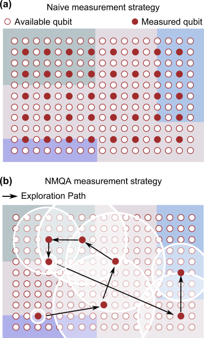
problem is to undertake a brute-force, “naive” strategy in which one uniformly measures sensor qubits across the array, depicted schematically in Fig. 1a. By extensively sampling qubit

locations in space repeatedly, one can build a map of the underlying noise fields through the collection of large amounts of measurement information. Evidently, the naive, brute-force

measurement approach is highly inefficient as it fails to recognize and exploit spatial correlations in the underlying noise field that may exist over a lengthscale that exceeds the

inter-qubit spacing. This is a particular concern in circumstances where qubit measurements are a costly resource, e.g., in time, classical communication bandwidth, or qubit utilization when

sensors are dynamically allocated. The NMQA framework shown in Fig. 1b stands in stark contrast, taking inspiration from the problem of simultaneous localization and mapping in robotic

control25,26,27,28,29,30,31,32,33. Here, the underlying spatial correlations of the noise are mapped using a learning procedure, which adaptively determines the location of the next,

most-relevant measurement to be performed based on past observations. With this approach, NMQA reduces the overall resources required for spatial noise mapping by actively exploiting the

spatial correlations to decide whether measurements on specific qubits provide an information gain. In our algorithmic implementation, at every iteration _t_, information about the true map

is contained in the state vector, _X__t_. Here, the word “state” refers to all quantities being inferred statistically from data, as opposed to an actual physical quantum state. Aside from

information about the true map that we denote _F__t_ ∈ _X__t_, the state vector, _X__t_, additionally contains information, _R__t_, which approximates spatial gradients on the true map. The

probability distribution of _X__t_ conditioned on data is called the posterior distribution, and it summarizes our best knowledge of the true map and its approximate spatial gradient

information, given past measurement outcomes. The key operating principle of NMQA is that we locally estimate the map value, \({F}_{t}^{(j)}\) (a qubit phase shift with a value between [0,

_π_] radians), before globally sharing the map information at the measured qubit _j_ with neighboring qubits _q_ ∈ _Q__t_ in the vicinity of _j_. The algorithm is responsible for determining

the appropriate size of the neighborhood, _Q__t_, parameterized by the length-scale value, \({R}_{t}^{(j)}\) (left panel, Fig. 2); accordingly, we may conceive \({R}_{t}^{(j)}\) as the

one-parameter mechanism to approximately learn local gradient information of the noise field. The combination of estimates of the state at each qubit and proxy local gradient information

allows for a more efficient mapping procedure than brute-force sampling over all qubits. In practice, _Q__t_ eventually represents the set of qubits in a posterior neighborhood at _j_ at the

end of iteration _t_, and this set shrinks or grows as inference proceeds over many iterations. We are ignorant, a priori, of any knowledge of \({R}_{t = 0}^{(j)}\). We set the prior

distribution over lengthscales to be uniform over an interval [_R_min, _R_max] where initial estimates take values between _R_min, the smallest inter-qubit spacing, and _R_max, as a multiple

of the maximal separation distance on the qubit array, in units of distance. In principle, any prior distribution over the lengthscales can be designed by practitioners. The collection of

map values and lengthscales, \({X}_{t}^{(j)}:=\{{F}_{t}^{(j)},{R}_{t}^{(j)}\}\), at every qubit, _j_ = 1, 2, …_d_, is depicted as an extended-state vector. We rely on an iterative

maximum-likelihood procedure within each iteration of the algorithm to solve the NMQA inference problem, as the size of the state–space generally impedes analytic solutions even in classical

settings32,34. In each iteration, we update _F__t_ assuming that _X__t_−1 is known, and subsequently _R__t_ based on _F__t_. This structure is unique, and NMQA manipulates the joint

probability distribution defined over _F__t_ and _R__t_, such that we numerically implement an iterative maximum-likelihood procedure using techniques known as particle filters (see below).

The final result of this first step in Fig. 2 is a posterior estimate of _X__t_, which represents our best knowledge given measurement data. This estimate is now passed to an adaptive

measurement scheduler, the NMQA controller, which attempts to maximize the information utility from each measurement. The NMQA controller adaptively selects the location _k_ for the next

physical measurement by choosing the region where posterior-state variance is maximally uncertain (Fig. 2, top–middle panel). The new measurement outcome, once collected, is denoted

\({Y}_{t+1}^{(k)}\) (a posterior-state variance is typically estimated using the properties of particles inside the filter35). Meanwhile, the posterior-state information at step _t_ is used

to generate data messages so that estimated map information can be shared with proximal neighboring qubits (Fig. 2, bottom–middle panel). The shared information is denoted by the set

\(\{{\hat{Y}}_{t+1}^{(q)},q\in {Q}_{t}\}\), where the posterior information in _Q__t_ at the end of _t_ is equivalent to information in _Q__t_+1 provided at the beginning of the next

iteration, _t_ + 1. The data messages \(\{{\hat{Y}}_{t+1}^{(q)}\}\) are taken as an input to the algorithm in a manner similar to a physical measurement. Jointly, the new actual physical

measurement, \({Y}_{t+1}^{(k)}\), and the set of shared information \(\{{\hat{Y}}_{t+1}^{(q)}\}\) form the inputs for the next iteration, _t_ + 1. Further technical information on the

overall NMQA implementation is presented in “Methods”. We approximate the theoretical nonlinear filtering problem embodied by NMQA using a class of techniques known as particle filters. In

each iteration of the NMQA algorithm, we must update information about the expected vectors _F__t_ and _R__t_ based on the latest measurement information acquired. This is a challenging data

inference problem that shares commonality with a host of other inference problems in science and engineering (such as robotic mapping36,37,38) involving nonlinear, non-Gaussian properties

or high-dimensional state spaces that are sparsely sampled. Particle filters are numerical approximation methods belonging to a general class of Sequential Monte Carlo algorithms used to

approximately solve the classical Bayesian inference problems under such conditions39. The prolific use of particle filters stems from their success in nonlinear filtering applications in

large state spaces of continuous random variables, relevant to the application considered here. In our application, the choice of a particle filter to implement core NMQA functionality

accommodates the nonlinear measurement model associated with the discretized outcomes given by projective qubit readout, and large state spaces defined over all possible maps and associated

lengthscales. Like many inference methods, particle filters use Bayes rule to solve an inference problem. Under Bayesian inference, the desired solution is a posterior distribution

representing the probability distribution of the inferred state conditioned on data. The defining feature of particle-filtering algorithms is that one sacrifices access to analytical

expressions for the moments of a posterior distribution (e.g., the mean). Instead, the posterior distribution is approximately represented as a discrete collection of weighted “particles”.

Each particle has two properties: a position and a weight. The position of the particle is effectively a hypothesis about the state _X__t_, i.e., a sample from the probability distribution

for _X__t_ given observed data. The weight specifies the likelihood or the importance of the particle in the estimation procedure. All weights are initially equal at step _t_ = 0, and after

receiving measurement data at each step, the particles are “re-sampled”. This means that the original set of particles at step _t_ is replaced by a set of “offspring” particles, where the

probability that a parent is chosen to represent itself in the next iteration (with replacement) is directly proportional to its weight. Over many iterations, only the particles with the

highest weights survive, and these surviving particles form the estimate of the distribution of _X__t_, given data in our algorithm. At any _t_, the estimate of _X__t_ can be obtained as the

first moment of the posterior particle distribution, and similarly, true state uncertainty is estimated from the empirical variance of the particle distribution. The efficacy of any

particle filter depends on how particle weights are computed, and many proposals to compute these weights exist. Further details on fundamental particle-filtering concepts and strategies to

compute particle weights are introduced in refs. 39,40 and restated in section 2C of Supplementary Information. We now provide a summary of the particle-filtering implementation used here,

and highlight modifications that are unique to NMQA. In each iteration, we update _F__t_ assuming that _X__t_−1 is known, and subsequently _R__t_ assuming _F__t_. This structure requires two

particle types inside NMQA’s particle filter: _α_ particles carry information about the full state vector, _X__t_, while _β_ particles discover the optimal information-sharing neighborhood

size, \({R}_{t}^{(j)}\), around qubit _j_. The two different types of particle sets are then used to manipulate the joint probability distribution defined over _F__t_ and _R__t_ to obtain an

estimate of _X__t_, which represents our best knowledge, given measurement data. Under the conditions articulated above, the NMQA filtering problem requires only two specifications: a prior

or initial distribution for the state vector, _X_0, at _t_ = 0, and a mechanism that assigns each particle with an appropriate weight based on measurement data. We take the approach where

particle weights are computed using a specific type of likelihood function for measurement, and a novel branching process, whose convergence properties can be analyzed41. Assuming a uniform

prior, we only need to define the global likelihood function incorporating both particle types. We label _α_ particles by the set of numbers {1, 2, …, _n__α_}; for each _α_ particle, we also

associate a set of _β_ particles denoted _β_(_α_), with _β_ taking values {1, 2, …, _n__β_}. Each _α_ particle is weighted or scored by a so-called likelihood function. This likelihood

function is written in notation as \({g}_{1}({\lambda }_{1},{Y}_{t}^{(j)})\), where _λ_1 is a parameter of the NMQA model and \({Y}_{t}^{(j)}\) makes explicit that only one physical

measurement at one location is received per iteration. A single _β_(_α_) particle inherits the state from its _α_ parent, but additionally acquires a single, uniformly distributed sample for

\({R}_{t}^{(j)}\) from the length-scale prior distribution. The _β_ particles are scored by a separate likelihood function, _g_2(_λ_2, _Q__t_), where _λ_2 is another parameter of the NMQA

model. Then the total likelihood for an (_α_, _β_(_α_)) pair is given by the product of the _α-_ and _β_-particle weights. The functions \({g}_{1}({\lambda }_{1},{Y}_{t}^{(j)})\) and

_g_2(_λ_2, _Q__t_) are likelihood functions used to score particles inside the NMQA particle filter, and their mathematical definitions can be found in the Supplementary Methods. These

functions are derived by representing the noise affecting the physical system via probability-density functions. The function \({g}_{1}({\lambda }_{1},{Y}_{t}^{(j)})\) describes measurement

noise on a local projective qubit measurement as a truncated or a quantized zero-mean Gaussian error model to specify the form of the noise-density function, with variance given by Σ_v_. The

function _g_2(_λ_2, _Q__t_) represents the probability density of “true errors” arising from choosing an incorrect set of neighborhoods while building the map. For each candidate map, the

value of the field at the center is extrapolated over the neighborhood using a Gaussian kernel. Thus, what we call “true errors” are the differences between the values of the true, spatially

continuous map and the NMQA estimate, consisting of a finite set of points on a map and their associated (potentially overlapping) Gaussian neighborhoods. We assume that these errors are

truncated Gaussian distributions with potentially nonzero means _μ__F_ and variances Σ_F_ over many iterations, as detailed in the Supplementary Methods. In general, the a priori theoretical

design of the likelihood function and its parameters depends on the choice of the measurement procedure and physical application. For static field characterization, we impose a tightly

regularized filtering procedure by setting low variance values relative to the initial state vector _X__t_=0 and machine precision. Low variance values correspond to physical assumptions

that bit-flip errors are unlikely, and high-frequency temporal noise is averaged away for large _T_, by setting Σ_v_ = 10−4. Further, we assume that the unknown field is continuous and

enables an approximation via overlapping Gaussian neighborhoods, by setting _μ__F_ = 0, Σ_F_ = 10−6. As with any filtering problem, one may alternatively consider an optimization routine

over design parameters and measurement protocols embodied by the likelihood functions, thereby removing all a priori knowledge of a physical application. The two free parameters, _λ_1, _λ_2

∈ [0, 1], are used to numerically tune the performance of the NMQA particle filter. Practically, _λ_1 controls how shared information is aggregated when estimating the value of the map

locally, and _λ_2 controls how neighborhoods expand or contract in size with each iteration. In addition, the numerically tuned values of _λ_1, _λ_2 ∈ [0, 1] provide an important test of

whether or not the NMQA sharing mechanism is trivial in a given application. Nonzero values suggest that sharing information spatially actually improves performance more than just locally

filtering observations for measurement noise. As _λ_1, _λ_2 → 1, the set \(\{{\hat{Y}}_{t+1}^{(q)}\}\), is treated as if they were the outcomes of real physical measurements by the

algorithm. However, in the limit _λ_1, _λ_2 → 0, no useful information sharing in space occurs, and NMQA effectively reduces to the naive measurement strategy. The information-sharing

mechanism described above also influences how the controller schedules a measurement at the next qubit location. At each _t_, the particle filter can access the empirical mean and variance

of the posterior distribution represented by the particles. In particular, the particle filter stores estimated posterior variance of the _β_ particles at qubit location _j_, if this

location was physically measured during the filtration until _t_. The ratio of the empirical variance of the _β_ particles to the posterior estimate of \({R}_{t}^{(j)}\), is then compared

for all qubit locations. The controller selects a location _k_ uniformly randomly between locations with the largest values of this ratio, corresponding to a location with the highest

uncertainty in neighborhood lengthscales. In the absence of information sharing (setting _λ_1, _λ_2 = 0), the controller effectively uniformly randomly samples qubit locations, and the

difference between NMQA and a deterministic brute-force measurement strategy is reduced to the random vs. ordered sampling of qubit locations. Detailed derivations for mathematical objects

and computations associated with NMQA, and an analysis of their properties using standard nonlinear filtering theory are provided in ref. 41. RESULTS Application of the NMQA algorithm using

both numerical simulations and real experimental data demonstrates the capabilities of this routine for a range of spatial arrangements of _d_ qubits in 1D or 2D. For the results reported in

this section, NMQA receives a single “0” or “1” projective measurement, \({Y}_{t}^{(j)}\), in each iteration _t_ and location _j_. We have also validated numerically that benefits persist

with continuous (classically averaged) measurement outcomes, where many single-qubit projective measurements, \(\{{Y}_{t}^{(j)}\}\), are averaged in each _t_ and _j_ in Fig. 5 of

Supplementary Figures. Our evaluation procedure begins with the identification of a suitable metric for characterizing mapping performance and efficiency. We choose a Structural SIMilarity

Index (SSIM)42, frequently used to compare images in machine-learning analysis. This metric compares the structural similarity between two images, and is defined mathematically in “Methods”.

It is found to be sensitive to improvements in the quality of images while giving robustness against, e.g., large single-pixel errors that frequently plague norm-based metrics for

vectorized images43,44. In our approach, we compare the true map and its algorithmic reconstruction by calculating the SSIM; a score of zero corresponds to ideal performance, and implies

that the true map and its reconstruction are identical. We start with a challenging simulated example, in which _d_ = 25 qubits are arranged in a 2D grid. The true field is partitioned into

square regions with relatively low and high values (Fig. 3a, left inset) to provide a clear structure for the mapping procedure to identify. In this case, the discontinuous change of the

field values in space means that NMQA will not be able to define a low-error candidate neighborhood for any qubits on the boundary. Both NMQA and naive are executed over a maximum of _T_

iterations, such that _t_ ∈ [1, _T_]. For simplicity, in most cases, we pick values of _T_ ≥ _d_ as multiples of the number of qubits, _d_, such that every qubit is measured the same integer

number of times in the naive approach, which we use as the baseline in our comparison. If _T_ < _d_, the naive approach uniformly randomly samples qubit locations. Both NMQA and the

naive approach terminate when _t_ = _T_, and a single-run SSIM score is calculated using the estimated map for each algorithm in comparison with the known underlying “true” noise map. The

average value of the score over 50 trials is reported as Avg. SSIM, and error bars represent 1 standard deviation (s.d.) for all data figures. The Avg. SSIM score as a function of _T_ is

shown in the main panel of Fig. 3a. For any choice of _T_, NMQA reconstructs the true field with a lower SSIM than the naive approach, indicating better performance. The SSIM score also

drops rapidly with _T_ when using NMQA, compared with a more gradual decline in the naive case. Increasing _T_ ≫ _d_ leads to not only an improvement in the performance of both algorithms,

but also a convergence of the scores as every qubit is likely to be measured multiple times for the largest values considered here. Representative maps for _T_ = 10 and _T_ = 75 measurements

under both the naive and NMQA mapping approaches are shown in Fig. 3b–e, along with a representative adaptive measurement sequence employed in NMQA in panel b. In both cases, NMQA provides

estimates of the map that are closer to the true field values, whereas naive maps are dominated by estimates at the extreme ends of the range, which is characteristic for simple

reconstructions using sparse measurements. It is instructive to represent these data in a form that shows the effective performance enhancement of the NMQA mapping procedure relative to the

naive approach; the upper-right inset in Fig. 3a reports the improvement in the reduction of the number of measurements required to reach a desired Avg. SSIM value. We perform linear

interpolation for each raw dataset in Fig. 3a, depicted using dashed lines in the main panel. The ratio of the interpolated data as a function of Avg. SSIM value is shown in the upper-right

inset of Fig. 3a (red solid). The interpolation process is repeated to obtain the difference between the maximum upper and minimum lower error trajectories (shaded gray) using error bars on

underlying raw data for these results. The shape of the performance improvement curve is linked to the total amount of information provided to both algorithms. At high Avg. SSIM scores on

the far right of the figure, both naive and NMQA algorithms receive very few measurements, and map reconstructions are dominated by errors. In the intermediate regime, a broad peak indicates

that NMQA outperforms brute-force measurement in reducing the total number of qubit measurements over a range of moderate-to-low Avg. SSIM scores for map reconstruction error, up to 7× for

Avg. SSIM = 0.1. Similar performance is achieved for a range of other qubit-array geometries and characteristics of the underlying field (Supplementary Figures). Near the origin at Avg. SSIM

 < 0.05, an extremely large number of measurements are required to achieve low Avg. SSIM scores. For _T_ → _∞_ and when all locations are measured, we theoretically expect the relative

performance ratio to approach unity for any true field. In empirical analysis, the relative improvement of NMQA to naive is based on projections of the interpolation procedure rather than

raw data. Our simulations at _T_ = 250 are being used to extrapolate at very low SSIM scores where the implied _T_ ~103 for both naive and NMQA; consequently, the resulting ratio is very

sensitive to a change in parameters of the interpolation procedure. An analytical, rather than empirical, investigation of NMQA’s convergence at low-error scores is presented in ref. 41. All

of our results rely on appropriate tuning of the NMQA particle filter via its parameters _λ_1 and _λ_2. Numerical tuning of these parameters is conducted for each _T_, and these data are

represented as a solid red curve in Fig. 3a. We also demonstrate that using fixed values for these parameters only marginally degrades performance, as indicated by the dashed line in the

upper-right inset of Fig. 3a. We now apply the NMQA mapping algorithm to real experimental measurements on qubit arrays. In Fig. 4, we analyze Ramsey experiments conducted on an array of

171Yb+ ions confined in a linear Paul trap, with trap frequencies _ω__x_,_y_,_z_/2_π_ ≈ (1.6, 1.5, 0.5) MHz. Qubits are encoded in the 2S1/2 ground-state manifold, where we associate the

atomic hyperfine states \(\left|F=0,{m}_{F}=0\right\rangle\) and \(\left|F=1,{m}_{F}=0\right\rangle\) with the qubit states \(\left|0\right\rangle\) and \(\left|1\right\rangle\),

respectively. State initialization to \(\left|0\right\rangle\) via optical pumping and state detection are performed using a laser resonant with the 2S1/2 − 2P1/2 transition near 369.5 nm.

Laser-induced fluorescence (corresponding to projections into state \(\left|1\right\rangle\)) is recorded using a spatially resolving EMCCD camera yielding simultaneous readout of all ions.

In this experiment, qubit manipulation is carried out using microwave radiation at 12.6 GHz delivered via an in-vacuum antenna to all qubits globally. The trapped ions experience an

uncontrolled (“intrinsic”), linear magnetic field gradient that produces spatially inhomogeneous qubit frequencies over the trap volume. When manipulated using a global microwave control

field, this results in a differential phase accumulation between qubits. The magnitude of the gradient is illustrated in Fig. 4a, superimposed on an image of six ions in the bright state

\(\left|1\right\rangle\), and is not observed to drift or vary on any timescale relevant to these experiments. We aim to probe this field gradient through the resulting qubit detuning and

associated differential phase accumulation throughout each measurement repetition. In this case, NMQA may be thought of as either an adaptive noise-mapping or calibration routine. A

preliminary Ramsey experiment, in which the interrogation time is varied, and fringes are observed, confirms that at an interrogation time of 40 ms, the accumulated relative phase in a

Ramsey measurement is <_π_ radians. A total of 25, 500 Ramsey measurements with a wait time of 40 ms are performed on all six ions in parallel. For each repetition, a standard

machine-learning image classification algorithm assigns a “0” (dark) or “1” (bright) to each ion based on a previously recorded set of training data. From averaging over repetitions, we

construct a map of the accumulated phase (and hence the local magnetic field inducing this phase) on each qubit, shown schematically in the left inset of Fig. 4b. We consider the field

extracted from this standard averaging procedure over all repetitions of the Ramsey experiment, at each ion location, as the “true” field against which mapping estimates are compared using

the SSIM score as introduced above. We employ the full set of 6 × 25,500 measurements as a data bank on which to evaluate and benchmark both algorithms. At each iteration, the algorithm

determines a measurement location in the array, and then randomly draws a single, discretized measurement outcome (0 or 1) for that ion from the data bank. The rest of the algorithmic

implementation proceeds as before. Accordingly, we expect that the naive approach must smoothly approach a SSIM score of zero as _T_ increases (Fig. 4b). In these experiments, we experience

a large measurement error arising from the necessary detection time of 750 μs associated with the relatively low quantum efficiency and the effective operating speed of the EMCCD camera.

Compensating this via extension of the measurement period leads to an asymmetric bias due to state decays that occur during the measurement process in ≈1.5 ms (\(\left|1\right\rangle \to

\left|0\right\rangle\)) and ≈30 ms (\(\left|0\right\rangle \to \left|1\right\rangle\)) under the laser power and quantization magnetic field strength used in our experiment. In our

implementation, neither NMQA nor the brute-force algorithm was modified to account for this asymmetric bias in the detection procedure, although in principle, the image classification

algorithm employed to determine qubit states from fluorescence detection can be expanded to account for this. Therefore, both NMQA and the naive approach are affected by the same detection

errors. Despite this complication, we again find that NMQA outperforms the naive mapping algorithm by a factor of 2–3 in the number of required measurements (Fig. 4b), with expected behavior

at the extremal values of Avg. SSIM. DISCUSSION In this work, we presented NMQA—a framework for adaptive learning where we reconstruct spatially varying parameters associated with qubit

hardware, derived from autonomously and adaptively scheduled measurements on a multi-qubit device. We developed an iterative, maximum-likelihood procedure implemented via a two-layer

particle filter to share state-estimation information between qubits within small spatial neighborhoods, via a mapping of the underlying spatial correlations of the parameter being measured.

An adaptive controller schedules future measurements in order to reduce the estimated uncertainty of the map reconstruction. We focused on the specific application of mapping an unknown

decoherence-inducing noise field, but this methodology could equally be applied to the characterization of nearly any device parameter subject to spatial inhomogeneities, and where

efficiency in measurement sampling is valued. This could include, for instance, calibration of qubit Rabi rates due to nonuniform coupling of devices to their control lines, or variations in

qubit frequencies arising from device-fabrication tolerances. Numerical simulations and calculations run on real experimental data demonstrated that NMQA outperforms a naive mapping

procedure by reducing the required number of measurements up to 3× in achieving a target map similarity score on a 1D array of six trapped ytterbium ions (up to 20× in a 2D grid of 25 qubits

using simulated data). Beyond these example demonstrations, the key numerical evidence for the correctness of NMQA’s functionality came from the observation that the tuned values of _λ_1,

_λ_2 ≫ 0 for all results reported here. Since numerically tuned values for these parameters were found to be nonzero, we conclude that information sharing in NMQA is nontrivial, and the

algorithm departs substantially from a brute-force measurement strategy. This contributes to the demonstrated improvements in Avg. SSIM scores when using NMQA in Figs. 3 and 4. Overall,

achieving suitable adaptive learning through NMQA requires that the (_λ_1, _λ_2) parameters are appropriately tuned using measurement datasets as part of a training procedure. To select

(_λ_1, _λ_2), we chose a (_λ_1, _λ_2) pair with the lowest expected error. In practice, one cannot calculate the true error as the true field is unknown. Additional numerical analysis shows

that tuned _λ_1, _λ_2 > 0 improves NMQA performance, and that this performance improvement gradually increases from the bottom-left to the top-right corner of the unit square away from

the case _λ_1 = _λ_2 = 0 (Fig. 1; Supplementary Figures) for a range of different noise fields with regularly spaced 1D or 2D configurations. This numerically observed gradual improvement in

performance as a function of _λ_1,2 → 1 suggests that theoretical approaches to deducing “optimal” regions for (_λ_1, _λ_2) may be possible. Meanwhile, in a specific application, a

practitioner may only have access to the real-time rate of change of state estimates and residuals, i.e., a particle filter generates a predicted measurement at location _j_, which can be

compared with the next actual measurement received at _j_. Monitoring the real-time rate of change of state estimates and/or residuals in a single run can be used to develop effective

stopping criteria to set (_λ_1, _λ_2) with minimal a priori knowledge of the physical system. If, for example, total preparation and measurement time is on the order of tens or hundreds of

microseconds, then an experiment of _T_ ~ 105 measurements takes a few minutes to complete. For ion traps, the relevant timescales for temporal drift in control fields are on the order of

hours. Meanwhile, run times for a single NMQA iteration are on the order of 1 ms in Python under typical operating conditions. Thus, it is possible to numerically tune _λ_1, _λ_2 for NMQA

using small _T_ measurements before proceeding with a desired experiment. Future work to speed up and integrate NMQA into low-level experimental control software appears promising as

particle filters do not require complicated linear algebra operations (e.g., matrix inversions), and enable rapid, parallel computations across particles. The particle-filtering structure of

NMQA presents as-yet unexplored opportunities in software execution to explore in-cycle tuning with run times on par with physical measurements. These extensions to the operability of NMQA

are active research areas. The framework we have introduced is flexible and can accommodate temporal variations in the system, such as drifts in the map and changes in the availability of

sensor qubits. Without a priori information about dynamics, the state-transition kernel is set to identity, and in this form, our assumption is that NMQA accommodates low-frequency drift

quasi-statically. Temporal dynamics rapid compared with the measurement cycle are generally averaged over, and ignored by the algorithm. In intermediate regimes, it may be possible to

accommodate fluctuations as measurement noise or error in our knowledge of a qubit’s given location. A formal spatiotemporal analysis with NMQA is the subject of future work, and combines a

nonidentity state-transition kernel with NMQA’s unique branching process. We have thus far presented a comparison of NMQA with a naive, brute-force measurement strategy, but it is also

possible to consider the error-scaling behavior under NMQA against a strengthened competing measurement procedure. For instance, it is possible to perform many measurements at each qubit

location in order to accurately (within a user-defined bound) establish the relevant mapped value for that qubit. One may gradually increase the number of simultaneous measurements at a

single location _j_ as 2, 3, …50, … measurements per iteration _t_ and so on, which means that NMQA takes in a classically post-processed measurement result rather than a “0” or “1”

projective measurement input. For a true field of Fig. 3, our investigations show that in the region of Avg. SSIM score ≈0.2, NMQA outperforms naive by a factor greater than ≫2 using 2–15

measurements per _t_, and is above unity in the regions 15–50 measurements per _t_ (Fig. 5; Supplementary Figures). In this case, determining where to measure next in order to build the map

still benefits from estimating lengt-scales to approximate local field gradient information; minimizing uncertainty in these estimated lengthscales informs an adaptive strategy. In the limit

that many qubit measurements are taken at every location (such as performing many averaged measurements in parallel), the naive brute-force measurement strategy essentially transitions from

an inference to an interpolation problem—i.e., given near-perfect knowledge of a finite-point set, we seek to approximately reconstruct an unknown continuous function in bivariate parameter

space. In this regime, the arrangement of qubits on a 2D plane affects the accuracy of the resulting reconstruction. One approach to this problem is to restrict physical measurements to a

subset of qubits within the register, requiring that the value of an unknown, continuous, spatially varying field must be inferred at the remaining set of unmeasured qubits. The study of

this approach, and comparison of the error-scaling behavior of an optimally constructed classical interpolant vs. NMQA is the subject of future work45. We are also excited to explore how

exploitation of hardware platforms in which qubit locations are not rigidly fixed during fabrication, such as with trapped ions, may allow sublattice spatial resolution by dynamically

translating individual qubits during the mapping procedure. Our work is part of an exciting new area of future study exploring the intersection between hardware architectures and control

solutions8,41 in NISQ-era quantum computers, and may also have bearing on distributed networks of quantum sensors. METHODS We summarize the structure of the NMQA algorithm in Algorithm 1

using a pseudocode representation. The first part of the algorithm consists of an initialization procedure, which ensures that all particles are sampled from the prior for extended-state

vector at _t_ = 0, giving _X_0. All particles are equally weighted before measurement data are received. For _t_ > 0, the function PropagateStates represents the transition-probability

distribution for Markov _X__t_, i.e., it represents identity dynamics, and is a placeholder for future extensions to model dynamical _F__t_. In each _t_, a single physical measurement is

received. This triggers a set of update rules for _F__t_ and _R__t_. We note that the state variables, _F__t_ and _R__t_, are updated in a specific order within each timestep _t_. The order

of these computations corresponds to the iterative maximum-likelihood approximation for the NMQA framework. ALGORITHM 1 NMQA PROCEDURE NMQA (_d_ qubit locations, _λ_1, _λ_2)  IF _t_ = 0 THEN

  PROCEDURE INITIALIZE (_X_0)    FOR _α_ ∈ {1, 2, …, _n__α_} DO     Initially sample \({x}_{0}^{(\alpha )} \sim {\pi }_{0}\)     Initially compute \({W}_{0}^{(\alpha )}=\frac{1}{{n}_{\alpha

}}\)    END FOR   END PROCEDURE  END IF  WHILE 1≤_t_ < _T_ DO   IF Controller THEN    \({j}_{t},{Y}_{t}^{({j}_{t})}\leftarrow\) CONTROLLER(_X__t_−1) ⊳ Qubit _j_, at _t_   END IF   FOR

_α_ ∈ {1, 2, …, _n__α_} DO    \(\{{x}_{t}^{(\alpha )}\}\leftarrow\) PROPAGATESTATES(\(\{{x}_{t-1}^{(\alpha )}\}\))    Update \({F}_{t}^{(\cdot ),(\alpha )}\) via

\(\{{Y}_{t}^{({j}_{t})},\{{\hat{Y}}_{t}^{({q}_{t})}\},{\lambda }_{1}\}\)    \(\{{\{{x}_{t},{W}_{t}\}}^{(\alpha ,{\beta }_{\alpha })}\}\leftarrow\) COMPUTEWEIGHTS(\(\{{x}_{t}^{(\alpha )}\}\))

   \(\{{x}_{t}^{(\alpha ,{\beta }_{\alpha })},\frac{1}{{n}_{\alpha }{n}_{\beta }}\}\leftarrow\) RESAMPLE(\(\{{\{{x}_{t},{W}_{t}\}}^{(\alpha ,{\beta }_{\alpha })}\}\))    Update

\({R}_{t}^{({j}_{t}),(\alpha )}\)    \(\{{\{{x}_{t},{W}_{t}\}}^{(\alpha )}\}\leftarrow\) COLLAPSE_β_(\(\{{x}_{t}^{(\alpha ,{\beta }_{\alpha })},\frac{1}{{n}_{\alpha }{n}_{\beta }}\}\))    

\(\{{x}_{t}^{(\alpha )},\frac{1}{{n}_{\alpha }}\}\leftarrow\) RESAMPLE(\(\{{\{{x}_{t},{W}_{t}\}}^{(\alpha )}\}\))   END FOR   \({\{{\hat{Y}}_{t+1}^{(q)}\}}_{q\in {Q}_{t+1}}\leftarrow\)

GENERATE\(\hat{Y}\)(Posterior _X__t_)  END WHILE END PROCEDURE FUNCTION COMPUTEWEIGHTS(\(\{{x}_{t}^{\alpha }\}\))  FOR _α_ ∈ {1, 2, …, _n__α_} DO   Compute\({\tilde{W}}_{t}^{(\alpha

)}={g}_{1}({\lambda }_{1},{Y}_{t}^{(j)})\)   \(\{{x}_{t}^{(\alpha ,{\beta }_{\alpha })}\}\leftarrow\) Generate _β_-layer   FOR _β__α_ ∈ {1, 2, …, _n__β_} DO    Compute

\({\tilde{W}}_{t}^{({\beta }_{\alpha }| \alpha )}={g}_{2}({\lambda }_{2},{Q}_{t})\)   END FOR   Normalize \({\tilde{W}}_{t}^{({\beta }_{\alpha }| \alpha )}\)  END FOR  Normalize

\({\tilde{W}}_{t}^{(\alpha )}\)  Compute \({W}_{t}^{(\alpha ,{\beta }_{\alpha })}={\tilde{W}}_{t}^{({\beta }_{\alpha }| \alpha )}{\tilde{W}}_{t}^{(\alpha )}\ \forall \{\alpha ,\{{\beta

}_{\alpha }\}\}\)  Return _n__α__n__β_ particles and weights \(\{{\{{x}_{t},{W}_{t}\}}^{(\alpha ,{\beta }_{\alpha })}\}\) END FUNCTION For each type of particle, the weights are computed

according to NMQA likelihood functions \({g}_{1}({\lambda }_{1},{Y}_{t}^{(j)})\) and _g_2(_λ_2, _Q__t_). These likelihood calculations are local about each qubit location, enabling NMQA to

receive multiple measurements in either the same or different locations in a single iteration _t_. Multiple measurements at one location improve the local map estimate \({F}_{t}^{(j)}\) at

_j_ via _g_1(_λ_1, ⋅) before the estimated \({F}_{t}^{(j)}\) is shared with proximal qubits. Multiple measurements at different but proximal locations improve the estimation of lengthscales

via _g_2(_λ_2, _Q__t_). This means that the net effect of parallelized measurements also depends on how these measurements sample an unknown field. We restrict our current scope to a single

physical measurement per iteration, and the effect of spatial sampling on functional reconstruction is the scope of a forthcoming paper. As typical of a standard particle filter, NMQA also

supports parallelization by ensuring that state transformations and weight calculations for each particle occur independently of other particles. Dynamical evolution and the computation of

_α-_ and _β_-particle weights are parallelizable for both _α_ and _β_ particles in software. While the normalization of particle weights represents a scalar rescaling of all particles in a

layer, this is computationally inexpensive. In our Python implementation of NMQA, a computational cost in sorting particles during resampling is incurred, and alternative resampling

techniques have been investigated in particle-filtering literature36,37,46. Nevertheless, the key strength of particle-filtering techniques is that they enable parallel computations while

avoiding matrix inversions that can be computationally expensive or ill-conditioned in numerical inference procedures, for example, Gaussian Process Regression47 or Kalman Filtering

techniques48. NMQA benefits from these advantages of standard particle filters. A detailed description of the nonlinear filtering problem represented by NMQA and its convergence properties

is provided in ref. 41. The correctness and convergence of typical particle filters are explored in the literature40,49, and we discuss it specifically for NMQA41. STRUCTURAL SIMILARITY

METRIC DEFINITION For all analyses, we use a risk metric called the Structural Similarity Index (SSIM)42. This metric is used to conduct optimization of NMQA parameters, and assess

performance relative to the naive measurement strategy. For two vectorized images _x_ and _y_, the metric is defined as $$s(x,y)=\frac{(2{\mu }_{x}{\mu }_{y}+{C}_{1})(2{\sigma

}_{xy}+{C}_{2})}{({\mu }_{x}^{2}+{\mu }_{y}^{2}+{C}_{1})({\sigma }_{x}^{2}+{\sigma }_{y}^{2}+{C}_{2})}$$ (1) $$\,\text{SSIM}\,(x,y):=| 1-s(x,y)|$$ (2) In the formula above, \({\mu

}_{i},{\sigma }_{i}^{2},i=x,y\) represent the sample estimates of the means and variances of the respective vectorized images, and _σ__x__y_ captures correlation between images. The term

_s_(_x_, _y_) is the key metric developed in ref. 42, and it includes arbitrary constants _C_1 = _C_2 = 0.01, which stabilize the metric for images with means or variances close to zero. The

ideal score given by _s_(_x_, _y_) is unity, and corresponds uniquely to the case _x_ = _y_. We report the absolute value of the deviations from the ideal score of unity, where the

direction of the deviation is ignored as given by SSIM(_x_, _y_). For our application, this SSIM(_x_, _y_) metric lies between [0, 1] (negative expected values of _s_(_x_, _y_) are not seen

in our numerical demonstrations). We report the average of SSIM(_x_, _y_) values over 50 trials as Avg. SSIM. DATA AVAILABILITY Access to the codebase and data required to reproduce all

figures is provided via http://github.com/qcl-sydney/nmqa without restrictions. REFERENCES * Yao, N. Y. et al. Scalable architecture for a room temperature solid-state quantum information

processor. _Nat. Commun._ 3, 800 (2012). Article  ADS  Google Scholar  * Monroe, C. et al. Large-scale modular quantum-computer architecture with atomic memory and photonic interconnects.

_Phys. Rev. A_ 89, 022317 (2014). Article  ADS  Google Scholar  * Veldhorst, M., Eenink, H. G. J., Yang, C. H. & Dzurak, A. S. Silicon CMOS architecture for a spin-based quantum

computer. _Nat. Commun._ 8, 1766 (2017). Article  ADS  Google Scholar  * Jones, N. C. Layered architecture for quantum computing. _Phys. Rev. X_ 2, 031007 (2012). Google Scholar  *

Kielpinski, D., Monroe, C. & Wineland, D. J. Architecture for a large-scale ion-trap quantum computer. _Nature_ 417, 709 (2002). Article  ADS  Google Scholar  * Franke, D. P., Clarke, J.

S., Vandersypen, L. M. K. & Veldhorst, M. Rentas rule and extensibility in quantum computing. _Microprocess. Microsys._ 67, 1–7 (2019). Article  Google Scholar  * Arute, F. et al.

Quantum supremacy using a programmable superconducting processor. _Nature_ 574, 505–510 (2019). Article  ADS  Google Scholar  * Ball, H., Nguyen, T., Leong, P. H. W. & Biercuk, M. J.

Functional basis for efficient physical layer classical control in quantum processors. _Phys. Rev. Appl._ 6, 064009 (2016). Article  ADS  Google Scholar  * Carvalho, A. et al. Software tools

for quantum control: Improving quantum computer performance through noise and error suppression. Preprint at https://arxiv.org/abs/2001.04060 (2020). * Brown, K. R., Aram, A. W. &

Chuang, I. L. Arbitrarily accurate composite pulse sequences. _Phys. Rev. A_ 70, 052318 (2004). Article  ADS  Google Scholar  * Merrill, J. T. & Brown, K. R. Progress in compensating

pulse sequences for quantum computation. In _Quantum Information and Computation for Chemistry_ (ed. Kais, S.) 241–294 (John Wiley, Sons, Inc., 2014). * Khodjasteh, K. & Viola, L.

Dynamically error-corrected gates for universal quantum computation. _Phys. Rev. Lett._ 102, 080501 (2009). Article  ADS  Google Scholar  * Soare, A. et al. Experimental noise filtering by

quantum control. _Nat. Phys_ 10, 825–829 (2014). Article  Google Scholar  * Paz-Silva, G. A. & Viola, L. General transfer-function approach to noise filtering in open-loop quantum

control. _Phys. Rev. Lett._ 113, 250501 (2014). Article  ADS  Google Scholar  * Kabytayev, C. et al. Robustness of composite pulses to time-dependent control noise. _Phys. Rev. A_ 90, 012316

(2014). Article  ADS  Google Scholar  * Gelb, A. _Applied Optimal Estimation_ (MIT Press, 1974). * Landau, I. D., Lozano, R., M’Saad, M. & Karimi, A. _Adaptive Control: Algorithms,

Analysis and Applications_ (Springer Science, Business Media, 2011). * Mavadia, S., Frey, V., Sastrawan, J., Dona, S. & Biercuk, M. J. Prediction and real-time compensation of qubit

decoherence via machine learning. _Nat. Commun._ 8, 14106 EP (2017). Article  ADS  Google Scholar  * Gupta, R. S. & Biercuk, M. J. Machine learning for predictive estimation of qubit

dynamics subject to dephasing. _Phys. Rev. Appl._ 9, 064042 (2018). Article  ADS  Google Scholar  * Majumder, S., de Castro, L. A. & Brown, K. R. Real-time calibration with spectator

qubits. _npj Quantum Inf._ 6, 1–9 (2020). Article  Google Scholar  * Cooper, A. et al. Time-resolved magnetic sensing with electronic spins in diamond. _Nat. Commun._ 5, 3141,

https://doi.org/10.1038/ncomms4141 (2014). Article  ADS  Google Scholar  * Brown, K. R., Kim, J. & Monroe, C. Co-designing a scalable quantum computer with trapped atomic ions. _npj

Quantum Inf._ 2, 16034, https://doi.org/10.1038/npjqi.2016.34 (2016). Article  Google Scholar  * Postler, L. et al. Experimental quantification of spatial correlations in quantum dynamics.

_Quantum_ 2, 90 (2018). Article  Google Scholar  * Hirose, M. & Cappellaro, P. Coherent feedback control of a single qubit in diamond. _Nature_ 532, 77–80 (2016). Article  ADS  Google

Scholar  * Cadena, C. et al. Past, present, and future of simultaneous localization and mapping: toward the robust-perception age. _IEEE Transac. Robot._ 32, 1309–1332 (2016). Article 

Google Scholar  * Bergman, N. Recursive bayesian estimation. _Department of Electrical Engineering, Linköping University, Linköping Studies in Science and Technology. Doctoral Dissertation_

579, 11 (1999). Google Scholar  * Stachniss, C. et al. Particle filters for robot navigation. _Found. Trends® Robot._ 3, 211–282 (2014). Article  Google Scholar  * Durrant-Whyte, H. &

Bailey, T. Simultaneous localization and mapping: part I”. _IEEE Robot. Autom. Mag._ 13, 99–110 (2006). Article  Google Scholar  * Bailey, T. & Durrant-Whyte, H. Simultaneous

localization and mapping (SLAM): part II. _IEEE Robot. Autom. Mag._ 13, 108–117 (2006). Article  Google Scholar  * Murphy, K. P. Bayesian map learning in dynamic environments. In _Advances

in Neural Information Processing Systems_ (eds Solla, S. A., Leen, T. K. & Müller, K.) 1015–1021. https://papers.nips.cc/book/advances-in-neural-information-processing-systems-12-1999

(Neural Information Processing Systems, 2000). * Andrew, H. Multi-robot simultaneous localization and mapping using particle filters. _Int. J. Robot. Res._ 25, 1243–1256 (2006). Article 

Google Scholar  * Thrun, S., Burgard, W. & Fox, D. _Probabilistic Robotics_ (MIT Press, 2005). * Thrun, S., Burgard, W. & Fox, D. A probabilistic approach to concurrent mapping and

localization for mobile robots. _Auton. Robots_ 5, 253–271 (1998). Article  Google Scholar  * Thrun, S. A probabilistic on-line mapping algorithm for teams of mobile robots. _Int. J.

Robotics Res._ 20, 335–363 (2001). Article  Google Scholar  * Bain, A. & Crisan, D. _Fundamentals of Stochastic Filtering_, Stochastic Modelling and Applied Probability (Springer, 2009).

* Beevers, K. R. & Huang, W. H. Fixed-lag sampling strategies for particle filtering SLAM. In _Proceedings 2007 IEEE International Conference on Robotics and Automation_ 2433–2438.

https://www.tib.eu/en/search/id/TIBKAT%3A555477428/Proceedings-Roma-Italy-10-14-April-2007/ (IEEE, 2007). * Grisettiyz, G., Stachniss, C. & Burgard, W. Improving grid-based slam with

Rao-Blackwellized particle filters by adaptive proposals and selective resampling. In _Proceedings of the 2005 IEEE International Conference on Robotics and Automation_ 2432–2437.

https://doi.org/10.1109/ROBOT.2005.1570477 (IEEE, Barcelona, Spain, 2005). * Poterjoy, J. A localized particle filter for high-dimensional nonlinear systems. _Monthly Weather Rev._ 144,

59–76 (2016). Article  ADS  Google Scholar  * Doucet, A., De Freitas, N. & Gordon, N. In _Sequential Monte Carlo Methods in Practice_ (eds Doucet, A., De Freitas, N. & Gordon, N.)

3–14 (Springer, 2001). * Bain, A. & Crisan, D. _Fundamentals of Stochastic Filtering_, Vol. 60 (Springer Science, Business Media, 2008). * Gupta, R. S. & Biercuk, M. J. Convergence

analysis for autonomous adaptive learning applied to quantum architectures. Preprint at https://arxiv.org/abs/1911.05752 (2019). * Wang, Z., Bovik, A. C., Sheikh, H. R. & Simoncelli, E.

P. Image quality assessment: from error visibility to structural similarity. _IEEE T. Image Process._ 13, 600–612 (2004). Article  ADS  Google Scholar  * Chen, Y., Garcia, E. K., Gupta, M.

R., Rahimi, A. & Cazzanti, L. Similarity-based classification: concepts and algorithms. _J. Machine Learn. Res._ 10, 747–776 (2009). MathSciNet  MATH  Google Scholar  * Wang, Z. &

Bovik, A. C. Mean squared error: love it or leave it? a new look at signal fidelity measures. _IEEE Signal Process. Mag._ 26, 98–117 (2009). Article  ADS  Google Scholar  * Gupta, R. S.,

Govia, L. C. & Biercuk, M. J. Integration of spectator qubits into quantum computer architectures for hardware tuneup and calibration. Preprint at https://arxiv.org/abs/2004.13059

(2020). * Li, T., Bolic, M. & Djuric, P. M. Resampling methods for particle filtering: classification, implementation, and strategies. _IEEE Signal Process. Mag._ 32, 70–86 (2015).

Article  ADS  Google Scholar  * Williams, C. K. & Rasmussen, C. E. _Gaussian Processes for Machine Learning_, Vol. 2, No. 3 (MIT Press, Cambridge, MA, 2006). * Grewal, M. S. _Kalman

Filtering_ (Springer, 2011). * Crisan, D. & Doucet, A. A survey of convergence results on particle filtering methods for practitioners. _IEEE T. Signal Process._ 50, 736–746 (2002).

Article  ADS  MathSciNet  Google Scholar  Download references ACKNOWLEDGEMENTS The authors thank V.M. Frey for proposing methods for single-ion-state detection using camera images, and S.

Sukkarieh, A.C. Doherty, and M. Hush for useful discussions. This work was partially supported by the ARC Centre of Excellence for Engineered Quantum Systems CE170100009, the US Army

Research Office under Contract W911NF-12-R-0012, and a private grant from H. & A. Harley. AUTHOR INFORMATION AUTHORS AND AFFILIATIONS * ARC Centre of Excellence for Engineered Quantum

Systems, School of Physics, The University of Sydney, Sydney, NSW, 2006, Australia Riddhi Swaroop Gupta, Claire L. Edmunds, Alistair R. Milne, Cornelius Hempel & Michael J. Biercuk

Authors * Riddhi Swaroop Gupta View author publications You can also search for this author inPubMed Google Scholar * Claire L. Edmunds View author publications You can also search for this

author inPubMed Google Scholar * Alistair R. Milne View author publications You can also search for this author inPubMed Google Scholar * Cornelius Hempel View author publications You can

also search for this author inPubMed Google Scholar * Michael J. Biercuk View author publications You can also search for this author inPubMed Google Scholar CONTRIBUTIONS The NMQA

theoretical framework and numerical implementations were devised by R.S.G. based on research directions set by M.J.B. R.S.G. and M.J.B. co-wrote the paper. A.R.M., C.L.E., and C.H. led all

experimental efforts and contributed to the paper draft. CORRESPONDING AUTHOR Correspondence to Riddhi Swaroop Gupta. ETHICS DECLARATIONS COMPETING INTERESTS The authors declare no competing

interests. ADDITIONAL INFORMATION PUBLISHER’S NOTE Springer Nature remains neutral with regard to jurisdictional claims in published maps and institutional affiliations. SUPPLEMENTARY

INFORMATION SUPPLEMENTARY INFORMATION RIGHTS AND PERMISSIONS OPEN ACCESS This article is licensed under a Creative Commons Attribution 4.0 International License, which permits use, sharing,

adaptation, distribution and reproduction in any medium or format, as long as you give appropriate credit to the original author(s) and the source, provide a link to the Creative Commons

license, and indicate if changes were made. The images or other third party material in this article are included in the article’s Creative Commons license, unless indicated otherwise in a

credit line to the material. If material is not included in the article’s Creative Commons license and your intended use is not permitted by statutory regulation or exceeds the permitted

use, you will need to obtain permission directly from the copyright holder. To view a copy of this license, visit http://creativecommons.org/licenses/by/4.0/. Reprints and permissions ABOUT

THIS ARTICLE CITE THIS ARTICLE Gupta, R.S., Edmunds, C.L., Milne, A.R. _et al._ Adaptive characterization of spatially inhomogeneous fields and errors in qubit registers. _npj Quantum Inf_

6, 53 (2020). https://doi.org/10.1038/s41534-020-0286-0 Download citation * Received: 29 October 2019 * Accepted: 21 May 2020 * Published: 12 June 2020 * DOI:

https://doi.org/10.1038/s41534-020-0286-0 SHARE THIS ARTICLE Anyone you share the following link with will be able to read this content: Get shareable link Sorry, a shareable link is not

currently available for this article. Copy to clipboard Provided by the Springer Nature SharedIt content-sharing initiative