Benchmarking the performance of bayesian optimization across multiple experimental materials science domains

ABSTRACT Bayesian optimization (BO) has been leveraged for guiding autonomous and high-throughput experiments in materials science. However, few have evaluated the efficiency of BO across a

broad range of experimental materials domains. In this work, we quantify the performance of BO with a collection of surrogate model and acquisition function pairs across five diverse

experimental materials systems. By defining acceleration and enhancement metrics for materials optimization objectives, we find that surrogate models such as Gaussian Process (GP) with

anisotropic kernels and Random Forest (RF) have comparable performance in BO, and both outperform the commonly used GP with isotropic kernels. GP with anisotropic kernels has demonstrated

the most robustness, yet RF is a close alternative and warrants more consideration because it is free from distribution assumptions, has smaller time complexity, and requires less effort in

initial hyperparameter selection. We also raise awareness about the benefits of using GP with anisotropic kernels in future materials optimization campaigns. SIMILAR CONTENT BEING VIEWED BY

OTHERS AUTONOMOUS MATERIALS DISCOVERY DRIVEN BY GAUSSIAN PROCESS REGRESSION WITH INHOMOGENEOUS MEASUREMENT NOISE AND ANISOTROPIC KERNELS Article Open access 19 October 2020 ACTIVE OVERSIGHT

AND QUALITY CONTROL IN STANDARD BAYESIAN OPTIMIZATION FOR AUTONOMOUS EXPERIMENTS Article Open access 27 January 2025 BAYESIAN OPTIMIZATION WITH ADAPTIVE SURROGATE MODELS FOR AUTOMATED

EXPERIMENTAL DESIGN Article Open access 03 December 2021 INTRODUCTION Autonomous experimental systems have recently emerged as the frontier for accelerated materials research. These systems

excel at optimizing materials objectives, e.g. environmental stability of solar cells or toughness of 3D printed mechanical structures, that are typically costly, slow, or difficult to

simulate and experimentally evaluate. While autonomous experimental systems are often associated with high sample synthesis rates via high-throughput experiments (HTE), they may also utilize

closed-loop feedback from machine learning (ML) during materials property optimization. The latter has motivated the integration of advanced lab automation components with ML algorithms.

Specifically, active learning1,2 algorithms have traditionally been applied to minimizing total experiment costs while maximizing machine learning model accuracy through hyperparameter

tuning. Their primary utility for materials science research, where experiments remain relatively costly, lies in an iterative formulation that proposes targeted experiments with regard to a

specific design objective based on prior experimental observations. Bayesian optimization (BO)3,4,5, one class of active learning methods, utilizes a surrogate model to approximate a

mapping from experiment parameters to an objective criterion, and provides optimal experiment selection when combined with an acquisition function. BO has been shown to be a data-efficient

closed-loop active learning method for navigating complex design spaces3,6,7,8,9,10. Consequently, it has become an appealing methodology for accelerated materials research and optimizing

material properties11,12,13,14,15,16,17,18,19,20,21,22 beyond state-of-the-art. The materials science community has seen successful demonstrations in performing materials optimization via

autonomous experiments guided by BO and its variants17,23,24,25,26,27. Naturally, previous work emphasized the ability to achieve materials optimization with fewer experimental iterations.

There have been very few quantitative analyses of the acceleration or enhancement resulting from applying BO algorithms and discussions on the sensitivity of BO performance to surrogate

model and acquisition function selection. Rohr et al.28, Graff et al.29, and Gongora et al.24 have evaluated the performance of BO using multiple surrogate models and acquisition functions

within specific electrocatalyst, ligand, and mechanical structures design spaces, respectively. However, comprehensive benchmarking of the performance of BO algorithms across a broad array

of experimental materials systems, as we present here, has not been done. Although one could test BO across various analytical functions or emulated materials design spaces25,30, empirical

performance evaluation on a broader collection of experimental materials science data is still necessary to provide practical guidelines. Optimization algorithms need systematic and

comprehensive benchmarks to evaluate their performance, and the lack of these could significantly slow down advanced algorithm development, eventually posing obstacles for building fully

autonomous platforms. Presented below, the benchmarking framework, practical performance metrics, datasets collected from realistic noisy experiments, and insights derived from a

side-by-side comparison of BO algorithms will allow researchers to evaluate and select their optimization algorithm before deploying it on autonomous research platforms. Our work provides

comprehensive benchmarks for optimization algorithms specifically developed for autonomous and high-throughput experimental materials research. Ideally, it provides insight for designing and

deploying Bayesian optimization algorithms that suit the sample generation rate of future autonomous platforms and tackle materials optimization in more complex design spaces. In this work,

we benchmark the performance of BO across five different experimental materials science datasets, optimizing properties of carbon nanotube-polymer blends, silver nanoparticles, lead-halide

perovskites, and additively manufactured polymer structures and shapes. We utilize a pool-based active learning framework to approximate experimental materials optimization processes. We

also adapt metrics such as enhancement factor and acceleration factor to quantitatively compare performances of BO algorithms against that of a random sampling baseline. We observe that when

utilizing the same acquisition functions, BO with Random Forest (RF)31,32,33 as a surrogate model has comparable performance to BO with Gaussian Process (GP)4 with automatic relevance

detection (ARD)34 that has an anisotropic kernel. They also both outperform commonly used BO with GP without ARD. Our discussion on surrogate models’ differences in their implicit

distributional assumptions, time complexities, hyperparameter tuning, and the benefits of using GP with anisotropic kernels yield deeper insights regarding surrogate model selection for

materials optimization campaigns. We also offer open-source implementation of benchmarking code and datasets to support the future development of such algorithms in the field. RESULTS

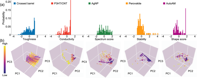
EXPERIMENTAL MATERIALS DATASETS As seen in Table 1, we have assembled a list of five materials datasets with varying sizes, dimensions _n_dim, and materials systems. These diverse datasets

are generated from autonomous experimental studies conducted by collaborators, and facilitate BO performance analysis across a broad range of materials. They contain three to five

independent input features, one property as materials optimization objective, and contain from a few tens to hundreds of data points. Based on their optimization objectives, the design space

input features in the datasets range from materials compositions to synthesis processing parameters, as seen in Supplementary Table 1–5. For consistency, each dataset has its optimization

problem formulated as global minimization. It should be noted that while all datasets were gathered from relatively high-throughput experimental systems, P3HT/CNT, AgNP, Perovskite, and

AutoAM had BO guiding the selection of subsequent experiments partially through the materials optimization campaigns. Across the datasets, the differences in the distribution of objective

values can be observed in Fig. 1(a) and the objective values are normalized for comparison purposes; the differences in the distribution of sampled data points in its respective materials

design space can be seen in Fig. 1(b). The five materials datasets in the current study are available in the following GitHub repository35. BAYESIAN OPTIMIZATION: SURROGATE MODELS AND

ACQUISITION FUNCTIONS Bayesian optimization (BO)3,4,5 aims to solve the problem of finding a global optimum (min or max) of an unknown objective function _g_: X* = arg \({\min

}_{{{{\bf{x}}}}}g({{{\bf{x}}}})\) where X ∈ _X_ and _X_ is a domain of interest in \({{{{\mathcal{R}}}}}^{{n}_{{{\text{dim}}}}}\). BO holds the assumption that this black-box function _g_

can be evaluated at any X ∈ _X_ and the responses are noisy point-wise observations (X, _y_), where _E_[_y_∣_g_(X)] = _g_(X). The surrogate model _f_ is probabilistic and consists of a prior

distribution that approximates the unknown objective function _g_, and is sequentially updated with collected data to yield a Bayesian posterior belief of _g_. Decision policies aimed to

find the optimum in fewer experiments are implemented in acquisition functions, which can use the mean and variance predicted at any X ∈ _X_ in the posterior to select the next observation

to be performed. The BO algorithm is comprised of both a surrogate model and an acquisition function. The surrogate models considered in this study are random forest (RF)31, Gaussian process

(GP) regression36, and GP with automatic relevance detection (ARD)5,34,36. * 1. To approximate the experience of a researcher with little prior knowledge of a materials design space, for

RF, we have hyperparameters applicable across all five datasets without loss of generality: _n_tree = 100 and bootstrap = True. Supplementary Figure 1 shows that _n_tree = 100 is a suitable

hyperparameter for RF surrogate models when applied to the five datasets. * 2. For hyperparameters of GP, we choose kernels from Matérn52, Matérn32, Matérn12, radial basis function (RBF),

and multilayer perceptron (MLP). The initial lengthscale for each kernel was set to unit length. * 3. For hyperparameters of GP ARD, we not only have the above kernel choices from GP, but

also use ARD, which allows GP to keep anisotropic kernels. The kernel function of GP then has individual characteristic lengthscales _l__j_5,34 for each of the input feature dimensions _j_.

As an example, in dimension _j_, Matérn52 kernel function between two points P, Q in design space would be $$k({{{{\bf{p}}}}}_{j},{{{{\bf{q}}}}}_{j})={\sigma }_{0}^{2}\cdot

(1+\frac{\sqrt{5}r}{{l}_{j}}+\frac{5{r}^{2}}{3{l}_{j}^{2}})\exp (-\frac{\sqrt{5}r}{{l}_{j}})$$ (1) where \(r=\sqrt{{({p}_{j}-{q}_{j})}^{2}}\), _σ_ is the standard deviation and _l__j_ is the

characteristic length scale. These characteristic length scales can be used to estimate the distance moved along _j_th dimension from the input values in the design space before the change

of objective values become uncorrelated with this feature. \(\frac{1}{{l}_{j}}\) is thus useful in understanding the sensitivity of objective value to input feature _j_. We then pair the

selected surrogate model with one of three acquisition functions, including expected improvement (EI), probability of improvement (PI), and lower confidence bound (LCB)

\({{{\mbox{LCB}}}}_{\overline{\lambda }}({{{\bf{x}}}})=-\hat{\mu }({{{\bf{x}}}})+\overline{\lambda }\hat{\sigma }({{{\bf{x}}}})\), where \(\hat{\mu }\) and \(\hat{\sigma }\) are the mean and

standard deviation estimated by surrogate model while \(\overline{\lambda }\) is an adjustable ratio between exploitation and exploration. In addition, these surrogate models, their

hyperparameters, and acquisition functions were chosen because they represent the majority of off-the-shelf options accessible, and are ones that have been widely applied to materials

optimization campaigns in the field. Our study provides a comprehensive test across the five datasets in order to reflect how each BO algorithm, resulting from the pairing above, performs

across many different materials science design spaces. GP and RF were also selected as examples to specifically illustrate how the differences in implicit distributional assumptions of

surrogate models could affect their predictions of the mean and standard deviation when selecting subsequent experiments and performance in BO. POOL-BASED ACTIVE LEARNING BENCHMARKING

FRAMEWORK Within each respective experimental dataset, the set of data points form a discrete representation of ground truth in the materials design space. Figure 2 shows the pool-based

active learning benchmarking framework we use to simulate materials optimization campaigns guided by BO algorithms in each materials system. The framework has the following properties: * 1.

It has the traits of an active learning study as it contains a machine learning model that is iteratively refined through subsequent experimental observation selection based on information

from previously explored data points. The framework is also adapted for BO, and emphasizes the optimization of materials objectives over building an accurate regression model in design

space. * 2. It is derived from pool-based active learning. Besides the randomly selected initial experiments, the subsequent experimental observations are selected from the total pool of

undiscovered data points (_x_, _y_) ∈ _D_, whose input features X are all made available for evaluation by the acquisition functions. The ground truth in the materials design space was

represented with a fixed number of discrete data points to resembles studies that have a known total number of experimental conditions to select from due to their equipment resolution

limitation. We chose such representation over a continuous emulator for the following reasons and concerns: * (a) In real research scenarios, materials design spaces are not completely

continuous due to noise and limitation in the resolution of equipment apparatus and experiment design. * (b) Because many materials datasets do not cover their design space evenly with at

high resolution, the fitted ground truth model would have greater variance in regions that were loosely covered by the training experimental dataset. As a result, even if we don’t consider

overfitting, the continuous emulator could have varied accuracy across its design space compared to real experimental ground truth, greatly affecting optimization results. * (c) To emulate

materials design spaces, selecting of models such as GP introduces smoothness assumptions into the design space, and thus during the benchmarking process could give great advantages to BO

algorithms with GP surrogate models sharing similar gaussianity assumptions. In Supplementary Figure 2 - 3, we show how such induced bias from different ground truth models affects the

evaluation of the performance of BO. * 3. At each learning cycle of the framework, instead of selecting a larger batch, only one new experiment is obtained. In our retrospective study, a

batch size of 1 was most applicable across five materials studies with varying dimensions and dataset sizes and allowed us to directly compare the impact of surrogate model and acquisition

function selection while keeping the same batch size. In real experimental setups, the exact tradeoff between batch size and cost of experiment parallelization should be determined by

researchers and their equipment apparatus limitations. Each BO algorithm is evaluated for 50 ensembles with 50 independent random seeds governing the initialization of experiments. The

aggregated performances of the BO algorithms derived from 50 averaged runs resulting from 10 random five-fold splits using the 50 original ensembles, is compared against a statistical random

search baseline, and we can quantitatively evaluate its performance via active learning metrics defined in the sections below. A detailed description of the framework and the calculation of

statistical random baselines can be seen in the Methods section. The simulated materials optimization campaigns were conducted on the Boston University Shared Computing Cluster (SCC) and

MIT Supercloud37, enabling the parallel execution of multiple optimization campaigns on individual computing nodes. OBSERVATION OF PERFORMANCE THROUGH CASE STUDY ON CROSSED BARREL DATASET

While the five datasets covered a breadth of materials domains, the relative performances of tested BO algorithms were observed to be quite consistent. The benchmarking results are thus

showcased using the Crossed barrel dataset24, which was collected by grid sampling the design space through a robotic experimental system while optimizing the toughness of 3D printed crossed

barrel structures. For the full combinatorial study including all types of GP kernels and acquisition functions, please kindly refer to Supplementary Figure 5–9 besides Fig. 3. As for the

performance metric, we use $$\,{{\mbox{Top}}} \% (i)=\frac{{{\mbox{number of top candidates discovered}}}}{{{\mbox{number of total top candidates}}}\,}\in [0,1]$$ (2) to show the fraction of

the crossed barrel structures with top 5% toughness that have been discovered by cycle _i_ = 1, 2, 3, …, _N_. Top% describes how quickly can a BO-guided autonomous experimental system could

identify multiple top candidates in a materials design space. Keeping multiple well-performing candidates allows one to not only observe regions in design space that frequently yield

high-performing samples but also have backup options for further evaluation should the most optimal candidate fail in subsequent evaluations. There are research objectives related to finding

any good materials candidate, yet in those cases, random selection could outperform optimization algorithms due to luck in a simple design space. Our objective of finding multiple or all

top-tier candidates is more applicable to experimental materials optimization scenarios and suitable for demonstrating the true efficacy and impact of BO. Figure 3 (a) illustrates learning

rates based on Top% metric and the following are observed: * 1. RF initially excels at lower learning cycles, while GP with ARD takes the lead after Top% = 0.46. Under the same acquisition

function, performance of RF as a surrogate model is often on par, if not slightly worse, when compared to the performance of GP with ARD. * 2. Both GP with ARD and RF outclass GP without

ARD. * 3. LCB\({}_{\overline{2}}\) typically outperform other LCB\({}_{\overline{\lambda }}\) acquisition functions that are biased towards overly exploration or exploitation as seen in

Supplementary Figure 5–9. These results enhance prior beliefs on acquisition strategy selection originated from theoretical studies38,39,40 and thus emphasize the importance of acquisition

strategies that balance exploration and exploitation for future studies. LCB\({}_{\overline{2}}\) at times even outperformed EI, which is a very popular acquisition function in many previous

materials optimization studies but has also been known to make excessive greedy decisions41,42,43. The performance of BO algorithms using the probability of improvement (PI) as acquisition

function has also been evaluated, but its performance was quite consistently worse than EI and therefore not the focus of discussion; this observation can be partially attributed to PI only

focusing on how likely is an improvement occurs at next experiment, but not considering how much improvement could be made during the evaluation. When trying to further compare the BO

algorithms with different surrogate models in this work, we would like to keep the acquisition function consistent. The same acquisition function LCB\({}_{\overline{2}}\) was thus used as a

representative acquisition function for surrogate model comparisons below because it has shown a decent balance of exploration and exploitation based on its benchmarking results. We would

like to highlight the relative performances of BO algorithms that utilize surrogate models GP ARD (Matérn52 kernel), RF, and GP (Matérn52 kernel). To quantify the relative performance, we

set Top% = 0.8 as a realistic goal to indicate we have identified 80% of the structures with top 5% toughness (Fig. 3a). For surrogate models paired with LCB\({}_{\overline{2}}\), we see

that GP with ARD and RF reach that goal by evaluating approximately 75 and 85 candidates out of the total of 600, whereas GP without ARD needs about 170 samples out of 600. Top% rises

initially as slowly as the random baseline because the surrogate models suffer from high variance in prediction, having only been trained with small datasets; Top% ramps up very quickly as

the model learns to become more accurate in identifying general regions of interest to explore; the rate of learning eventually slows down at high learning cycles because the local

exploitation for the global optimum has exhausted most if not all top 5% toughness candidates, and the algorithms therefore switch to exploring sub-optimal regions. Therefore, it can be

assumed that the most valuable regions to examine performance is before each curve reaches Top% = 0.8 and Top% = 0.8 can be used as a realistic optimization goal. To quantify the

acceleration of discovery from BO, we adapt two other metrics similar to the ones from Rohr et al.28. Both compared to a statistical random baseline, Enhancement Factor (EF)

$$\,{{\mbox{EF}}}(i)=\frac{{{\mbox{Top}}}{ \% }_{{{\mbox{BO}}}}(i)}{{{\mbox{Top}}}{ \% }_{{{\mbox{random}}}}(i)}$$ (3) shows how much improvement in a metric one would receive at cycle _i_,

and Acceleration Factor (AF) $$\,{{\mbox{AF}}}({{\mbox{Top}}} \% =a)=\frac{{i}_{{{\mbox{BO}}}}}{{i}_{{{\mbox{random}}}}}$$ (4) is the ratio of cycle numbers showing how much faster one could

reach a specific value Top%(_i_BO) = Top%(_i_random) = _a_ ∈ [0, 1]. The aggregated performance of BO algorithms is further quantified via EF and AF curves in Fig. 3(b, c): starting off

with small EFs or AFs before the surrogate model gains more accuracy; reaching absolute EFmax and AFmax of up to 8 × . Eventually, the learning algorithms show diminishing returns from an

information gain perspective as we progress deeper into our optimization campaigns during pool-based active learning. We observe that for the two BO algorithms both with the same acquisition

function LCB\({}_{\overline{2}}\) but different surrogate models GP ARD and RF, they reach EFmax at different learning cycles and AFmax at different Top%, both corresponding to the switch

of best-performing algorithm around Top% = 0.46. RF: LCB\({}_{\overline{2}}\) clearly excels at lower learning cycles, yet GP ARD: LCB\({}_{\overline{2}}\) takes the lead and would reach

Top% = 0.8 with fewer experiments. Therefore, these results objectively show that optimal BO algorithm selection varies with the assigned experiment budget and specific optimization task28.

Since we identified two BO algorithms, RF: LCB\({}_{\overline{2}}\) and GP ARD: LCB\({}_{\overline{2}}\), to have comparable performance, we wanted to further investigate how similar their

optimization paths were in the design space when starting from the same initial experiments. In Fig. 3(d), we use the Jaccard similarity index to quantify the similarity in optimizations

paths. Jaccard similarity, \(J=\frac{| A\cap B| }{| A\cup B| }\), is the size of the intersection divided by the size of the union of two finite sample sets; specifically in our benchmarking

study, using the same 50-ensemble runs that generated Fig. 3(a), we can calculate Jaccard similarity value _J_(_i_) at each learning cycle _i_, where _A_(_i_) is the set of data points

sequential collected at each learning cycle during an optimization path guided by BO algorithm GP ARD: LCB\({}_{\overline{2}}\), and _B_(_i_) is that of using RF: LCB\({}_{\overline{2}}\).

As baselines, we have also drawn what the Jaccard similarity value would look like between two optimization paths that begin with the same initial experiments and statistically have the

least overlap or most overlap. When _i_ = 1 or 2, the same initial experiments are given to the two BO algorithms, and _J_ = 1. When 2 < _i_ < 18, we can see that the Jaccard

similarity value drops as quickly as the statistically least overlapping paths, indicating that despite the fact that GP with ARD and RF were trained on the same initial experiments at the

onset, they follow very different paths in the materials design space. This behavior indicates that, despite achieving comparable performance, they exploit the underlying physics differently

by virtue of the choice of experiments. When _i_ ≥ 18, the general trend is that _J_ increases with _i_, indicating that the paths chosen by the two algorithms gradually start to have some

overlap as they move towards finding crossed barrels structures with high toughness. Recall both algorithms reached Top% = 0.8 between 75 to 85 learning cycles in Fig. 3(a), and between

those learning cycles, we observe that _J_ is approximately between 0.27–0.33, still considerably far from _J_ = 1. This observation shows that while both algorithms have comparable

performance in the task of finding crossed barrel structures with good toughness, due to their different choice of surrogate models, their paths towards discovering optimum can differ

considerably. In addition, the Jaccard similarity value does not increase monotonically, and a significant drop can be seen in _J_ such as one around _i_ = 50, which coincides with the

learning cycles where GP ARD: LCB\({}_{\overline{2}}\) overtook RF : LCB\({}_{\overline{2}}\) as best performing algorithm in Fig. 3(a). Since the two algorithms used the same acquisition

function, this observation shows that while in general the optimization paths of the two algorithms have more overlap over time, occasional divergent paths still take place because the two

algorithms have a considerable difference in gathered data used to learn their surrogate models and how their surrogate models predict mean and standard deviation. GP ARD :

LCB\({}_{\overline{2}}\) and RF : LCB\({}_{\overline{2}}\) started at the same two initial experiments and use the same acquisition function, and the only difference is the surrogate model

used. Thus, the divergence and convergence in optimization paths can be again primarily attributed to GP ARD and RF exploiting underlying physics of crossed barrel structure differently.

Figure 3(d) highlights the impact of different surrogate model selection beyond final performance, and to provide better guidelines to future research, inspires us to further investigate the

role of surrogate models. COMPARISON OF PERFORMANCE ACROSS DATASETS To further assess the performance of BO, similar optimization campaigns were conducted for the P3HT/CNT, AgNP, AM ARES,

and Perovskite datasets. Across most, if not all, of the investigated datasets, it was observed quite consistently that the performance of BO algorithms using GP with ARD and RF as surrogate

models were comparable, and both outperform those using GP without ARD in most datasets. To illustrate, in Fig. 4, we show such relative performance using normalized EFmax of BO algorithms

same acquisition function LCB\({}_{\overline{2}}\) but with different surrogate models across all five datasets. In addition to the observation on relative performance, we also observe that

BO algorithms with RF and GP ARD as a surrogate models also have plenty of overlap between their 5th to 95th percentile across five datasets, further indicating their similarity in

performance. We also observe the variance of EFmax for RF is on average lower than those for GPs. This phenomenon can be attributed to RF being an ensemble model, where the high variances

from many single decision trees are mitigated through aggregation, resulting in a model with relatively low bias and medium variance32,44. GP with anisotropic kernels (GP ARD) is thus shown

to be a great surrogate model across most materials domains, with RF being a close second, and both proving to be robust models for future optimization campaigns. Notably, EFmax of the other

four datasets were in the 2 × to 4 × range as seen in Supplementary Figure 4, which is noticeably lower than the EFmax of the crossed barrel dataset in Fig. 3(b). The difference in the

absolute EFmax can be attributed to the data collection methodology of the individual datasets. While the crossed barrel dataset was collected using a grid sampling approach, the other four

studies were collected along the path of a BO-guided materials optimization campaign. Therefore, these four datasets were smaller in size and possessed an intrinsic enhancement and

acceleration within their datasets. As a result, it is reasonable that these datasets demonstrate lower EFs, AFs during benchmarking. Noticeably, the Perovskite dataset had the most

intrinsic acceleration because its next experimental choice was guided by BO infused with probabilistic constraints generated from DFT proxy calculations of the environmental stability23 of

perovskite. As a result, the optimization sequence to be chosen in that study is already narrowed down to a more efficient path from initial experiments to final optimum, making the random

baseline to appear arbitrarily much worse. Another interesting observation is how the performance of BO with GP without ARD (isotropic kernels) as a surrogate model catches up with those of

BO with GP ARD and RF in Perovskite and AutoAM dataset where the design space has an already “easier" path towards the optimum. That is, when materials design space is relatively

simple, GP without ARD can serve as an equally good surrogate model in BO compared to GP ARD and RF. Despite the differences described above, we observe that absolute EFmax > 1 across

five datasets, indicating that performance enhancements of BO over a random baseline still exists even in such uneven search spaces. The results again show that BO is a very effective tool

for experimental selection in materials science. The hypothesis that the lower EFmax are caused by intrinsic acceleration and enhancement resulting from the dataset collection process can be

verified by collecting a subset from the uniform grid sampled crossed barrel dataset. This subset is collected by running BO algorithm GP: EI until all candidates with top 5% toughness are

found, representing an “easier" path towards optimums, and therefore carries intrinsic enhancement and acceleration. We run the same benchmarking framework on this subset, and observe

that EFmax is reduced, as seen in Supplementary Figure 4. DISCUSSION In this section, we further compare GP ARD, RF, and GP as surrogate models in BO under the context of autonomous and

high-throughput materials optimization. BO algorithms with GP-type surrogate models have been extensively used in many published materials studies and have shown to be robust models suitable

for most optimization problems in materials science based on our benchmarking results in Fig. 3 and Supplementary Figure 4. Meanwhile, RF is a close second alternative to GP in BO for

future HT materials optimization campaigns when considering the factors below. To briefly summarize, RF is free from distribution assumptions in comparison to GP-type models. In general, it

is quicker to train due to smaller time complexity, and requires less effort in initial hyperparameter selection. The lack of extrapolation power in RF can also be partially mitigated via

initial sampling strategies. We first highlight the difference between GP and RF during the prediction of mean and standard deviation, where GPs rely on heavy distributional assumptions

while RF is distribution-free. GP, whether anisotropic or isotropic, is essentially a distribution over a materials design space such that any finite selection of data points in this design

space results in a multivariate Gaussian density over any point of interest. For the selection of a new data point as the next experiment, its predicted mean and standard deviation are all

part of such a gaussian distribution constructed from previous experiments. Therefore, the predicted means and standard deviations of GPs from their posteriors carry gaussianity assumptions

and can be interpreted as statistical predictions based on prior information. Meanwhile, an RF is an ensemble of decision trees that have slight variation due to bootstrapping. For RF,

prediction of objective value and the standard deviation at a new point in materials space is an aggregated result, namely averaging44 the values from all its decision trees’ respective

predictions. Compared to those of GPs, the predicted means and standard deviations of RFs do not have distributional assumptions, and can be interpreted as empirical estimates. If rarely the

ground truth of a materials design space indeed satisfied the gaussianity assumptions, then GP type surrogate models could have an advantage over RF in BO as seen in Supplementary Figure

2-3. However, commonly seen phase changes and exponential relations from thermodynamics often introduce measurements with piece-wise constants or with orders of magnitude changes within

neighboring regions of materials design space. Whether these are new findings or outliers, they should be of specific interest to experimentalists. These results are typically smoothed out

in the GP surrogate model to satisfy its distributional assumptions. The decision trees of RF would be able to capture these points more accurately and reflect their influences on future

predictions. While both RF and GP are both suitable surrogate models, we would like to highlight their fundamental differences when fitting materials domain with unknown distributional

assumption. We next discuss the difference in time complexities of GP and RF as surrogate models. Across five datasets in this study, starting from the same initial experiments and using the

same acquisition function LCB\({}_{\overline{2}}\), the ratio of average running time to finish benchmarking framework between the three surrogate models is _t_RF: _t_GP: _t_GP ARD = 1: 

1.14: 1.32. For the fitting, we have time complexities \({t}_{{{\text{RF}}}}={{{\mathcal{O}}}}(nlog(n)\cdot {n}_{{{\text{dim}}}}\cdot {n}_{{{\text{tree}}}}) <

{t}_{{{\text{GP}}}}={{{\mathcal{O}}}}({n}^{{{\text{3}}}}+{n}^{{{\text{2}}}}\cdot {n}_{{{\text{dim}}}})\)45,46,47, where _n_ is the number of training data, _n_dim is the design space

dimension, _n_tree is the number of decision trees kept in the RF model. The higher computational complexity of the GP model is mostly due to the process of calculating the inverse of an _n_

by _n_ matrix during its training process, and keeping anisotropic kernels has added extra computational time. In our study, the datasets are relatively small in size _n_, and therefore the

time complexity \({{{\mathcal{O}}}}({n}^{{{\text{3}}}})\) of GP was less troublesome while that of RF is mostly dominated by \({{{\mathcal{O}}}}({n}_{{{\text{dim}}}}\cdot

{n}_{{{\text{tree}}}})\). However, if our datasets had sizes of order 105 or 106, the amount of computational resources to run BO algorithms with GP-type surrogate models could quickly

become intractable due to cubic complexity to _n_ and a significantly larger difference in computation speed between RF and GPs would be easily noticeable. As a result, despite being a

better performing surrogate model type, GP could be less preferred compared to RF in real-time optimization problems when there is a time limit for selecting the next set of conditions48.

For HT materials research, with increased application of automation, time used in generating samples will eventually match with the time used in suggesting new experiments. Thus, if we aim

to have a fast and seamless feedback loop between running BO and performing high-throughput materials experiments, then RF could have a potential advantage over GP-type surrogate models when

considering the tradeoff between performance and time complexity. We last discuss the effort required hyperparameter tuning of a surrogate model during optimization. While RF has

potentially more hyperparameters such as _n_tree, max depth, and max split to select, it is less penalized for sub-optimal choice of hyperparameters compared to GP. In this study, across

five datasets, as long as sufficient _n_tree were used in RF, its regression accuracy is comparable to that of RF with larger _n_tree as seen in Supplementary Figure 1. Other hyperparameters

of RF such as max depth or a minimum number of samples for leaf node either have had less of an impact or are too arbitrary to decide at the start of BO campaign in a specific materials

domain. Meanwhile, besides the implicit distribution assumption of using a GP type surrogate model, a kernel (covariance function) of GP specifies a specific smoothness prior on the domain.

Choosing a kernel that is incompatible with the unknown domain manifold could significantly slow down optimization conversion due to loss of generalization. For example, the Matérn52 kernel

analytically requires the fitted GP to be 2 times differentiable in the mean-square sense4, which can be difficult to verify for unknown materials design spaces. Selecting such a kernel

could introduce extra domain smoothness assumptions to an unfamiliar design space, as we often have limited data to make confident distribution assumptions of the domain at optimization

onset. Instead of devoting a nontrivial experimental budget to finding the best kernel for GP using adaptive kernels49, automating kernel selection50 or keeping a library of kernels

available via online learning, RF is an easier off-the-shelf option that allows one to make fewer structural assumptions about unfamiliar materials domains. If a GP-type surrogate model is

still preferred, a Multilayer Perceptron (MLP) kernel51 mimicking smoothness assumption-free neural networks would be suggested as it has comparable performance to other kernels as seen in

Supplementary Figure 5-9. Admittedly, our benchmarking framework might have given RF a slight advantage by discretizing the materials domain through actively acquiring a new data point at

each cycle and limiting the choice of next experiments within the pool of undiscovered data points. However, the crossed barrel dataset has a sampling density, size, and range within its

design space sufficient to cover its manifold complexity. A drawback of RF is that it performs poorly in extrapolation beyond the search space covered by training data, yet in the context of

materials optimization campaigns, this disadvantage can be mitigated by clever design of initial experiments, namely using sampling strategies like Latin hypercube sampling (LHS). In this

way, we can not only preserve the pseudo-random nature of selecting initial experiments but also cover a wider range of data in each dimension so that the RF surrogate model would not have

to often extrapolate to completely unknown regions. We thus believe that when paired with the intuitive tuning of LCB’s weights to adjust exploration and exploitation, RF warrants more

consideration as an alternative to GP ARD as a surrogate model in BO for general materials optimization campaigns at early stages. We would like to lastly raise awareness about the benefits

of using GP with anisotropic kernels over GP with isotropic kernels in future materials optimization campaigns. As mentioned earlier, ARD allows us to utilize individual lengthscales for

each input dimension _j_ in the kernel function of GP, which are subsequently optimized along with learning cycles. These lengthscales in an anisotropic kernel provide a “weight" for

measuring the relative relevancy of each feature to predicting the objective, i.e. understanding the sensitivity of objective value to each input feature dimension. The reason GP without ARD

shows worse performance is as follows: it will have a single lengthscale in an isotropic kernel as a scaling parameter controlling GP’s kernel function, which is at odds with the fact that

each input feature has its distinct contribution to the objective. Depending on how different each feature is in nature, range, and units, e.g. solvent composition vs. printing speed, using

the same lengthscale in the kernel function for each feature dimension could provide unreliable predictive results. The materials optimization objective naturally has different sensitivities

to each input variable, and thus it is rationale then, that the “lengthscale" parameter inside the GP kernel should be independent. In Fig. 4, the noticeable improvements of using an

anisotropic kernel can be seen in the relative lower performance of GP without ARD compared to that of GP with ARD. While data normalization can partially alleviate the problem, how it is

conducted is highly subject to a researcher’s choice, and therefore we would like to raise awareness of the benefits of using GP with anisotropic kernels. In addition, the lengthscales from

the kernels of GP with ARD provides us with more useful information about the input features. These lengthscale values have been used for removing irrelevant inputs4, where high _l__j_

values imply low relevancy input feature _j_. In the context of materials optimization, we find the following use of ARD especially useful: ARD could identify a few directions in the input

space with specially high “relevance.” This means that if we train GP with ARD on input data with their original units and without normalization, once we extract the length scale of each

feature _l__j_, our GP model in theory should not be able to accurately extrapolate more than _l__j_ units away from collected observations in _j_th dimension. Thus, _l__j_ suggests the

range of next experiments to be performed in the _j_th dimension of the materials design space. It also infers a suitable sampling density in each dimension in the experimental setting. When

a particular input feature dimension has a relative small _l__j_ or large \(\frac{1}{{l}_{j}}\), it means that for a small change in objective value, we would have a relatively large change

in the location within this input feature dimension; thus, the sampling density or resolution in this dimension should be high enough to capture such sensitivity. Previous studies have

considered using information extracted from these length scales for even more advanced analysis and variable selection52. At the expense of computation time tolerable in the context of

materials optimization campaigns, an anisotropic kernel provides not only a better generalizable GP model but also useful information in analyzing input feature relevancy at each learning

cycle. For the above mentioned reasons, it would be great practice for researchers to emphasize their use of GP with anisotropic kernels over GP with isotropic kernels as surrogate models

during materials optimization campaigns. In conclusion, we benchmarked the performance of BO algorithms across five different experimental materials science domains. We utilize a pool-based

active learning framework to approximate experimental materials optimization processes, and adapted active learning metrics to quantitatively evaluate the enhancement and acceleration of BO

for common research objectives. We demonstrate that when paired with the same acquisition functions, RF as a surrogate model can compete with GP with ARD, and both outperform GP without ARD.

In the context of autonomous and high-throughput experimental materials research, GP with anisotropic kernel has shown to be more robust as a surrogate model across most design spaces, yet

RF also warrants more consideration because of it being free from distribution assumptions, having lower time complexities, and requiring less effort in initial hyperparameter selection. In

addition, we raise awareness about the benefits of using GP with anisotropic kernels over GP with isotropic kernels in future materials optimization campaigns. We provide practical

guidelines on surrogate model selection for materials optimization campaigns, and also offer open-source implementation of benchmarking code and datasets to support future algorithmic

development. Establishing benchmarks for active learning algorithms like BO across a broad scope of materials systems is only a starting point. Our observations demonstrate how the choice of

active learning algorithms has to adapt to their applications in materials science, motivating more efficient ML-guided closed-loop experimentation, and will likely directly result in a

larger number of successful optimization of materials with record-breaking properties. The impact of this work can be extended to not only other materials systems, but also a broader scope

of scientific studies utilizing closed-loop and high-throughput research platforms. Through our benchmarking effort, we hope to share our insights with the field of accelerated materials

discovery and motivate a closer collaboration between ML and physical science communities. METHODS PREDICTION BY SURROGATE MODELS AND ACQUISITION FUNCTIONS In order to estimate the mean

\(\hat{\mu }({{{{\bf{x}}}}}_{* })\) and standard deviation \(\hat{\sigma }({{{{\bf{x}}}}}_{* })\) of predicted objective value at a previously undiscovered observation X* in design space:

For a Gaussian process (GP), it assumes a prior over the design space that is constructed from already collected observations (x_i_, _y__i_), _i_ = 1, 2, . . . , _n_. This prior is the

source of implicit distributional assumptions, and when an undiscovered new observation (\({\mathbf{x}}_\ast\), \({{y}}_\ast\)) is being considered during a noisy setting (_σ_ = 0.01), the

joint distribution between the objective values of collected data \({{{\bf{y}}}}\in {{{{\mathcal{R}}}}}^{{{\text{n}}}}\) and \({{y}}_\ast\) is $$\left[\begin{array}{l}{{{\bf{y}}}}\\ {y}_{*

}\end{array}\right] \sim {{{\mathcal{N}}}}\left(0,\left[\begin{array}{ll}K+{\sigma }^{2}I&{K}_{* }^{T}\\ {K}_{* }&{K}_{* * }\end{array}\right]\right).$$ (5) _K_ is the covariance

matrix of the input features _X_ = {X_i_∣_i_ = 1, 2, . . . , _n_}; \({{K}}_\ast\) is the covariance between the collected data and new input feature \({\mathbf{x}}_\ast\); \({{K}}_{\ast

\ast}\) is the covariance between the new data. For each of the covariance matrices, _K__p__q_ = _k_(X_p_, X_q_), where _k_ is the kernel function, whether isotropic or anisotropic, used in

GP. Then from the posterior, we have estimates \({{K}}_\ast\) $$\hat{\mu }({{{\bf{x}}}})={y}_{* }={K}_{* }{[K+{\sigma }^{2}I]}^{-1}{{{\bf{y}}}}$$ (6) and covariance matrix $$cov({y}_{*

})={K}_{* * }-{K}_{* }{[K+{\sigma }^{2}I]}^{-1}{K}_{* }^{T}$$ (7) The standard deviation value \(\hat{\sigma }({{{\bf{x}}}})\) can be obtained from the diagonal elements of this covariance

matrix. For a random forest (RF), let \({\hat{h}}_{k}({{{{\bf{x}}}}}_{* })\) denote the prediction of objective value from the _k_th decision tree in the forest, _k_ = 1, 2, . . . , _n_tree,

then $$\hat \mu ({{\mathbf{x}}_*}) = \dfrac{1}{{{n_{{\rm{tree}}}}}}\sum\limits_{k = 1}^{{n_{{\rm{tree}}}}} {{{\hat h}_{\rm{k}}}} ({{\mathbf{x}}_*})$$ (8) and $$\hat{\sigma

}({{{{\bf{x}}}}}_{* })=\sqrt{\frac{\mathop{\sum }\limits_{k = 1}^{{n}_{{{\text{tree}}}}}{({\hat{h}}_{k}({{{{\bf{x}}}}}_{* })-\hat{\mu }({{{{\bf{x}}}}}_{* }))}^{2}}{{n}_{{{\text{tree}}}}}}$$

(9) The median or other variations could also be used in future studies to aggregate the predictions for potential improvement in robustness44. We tested three acquisition functions in our

study, including expected improvement (EI), probability of improvement (PI), and lower confidence bound (LCB). $$\,{{\mbox{EI}}}\,({{{\bf{x}}}})=({y}_{{{\text{best}}}}-\hat{\mu

}({{{\bf{x}}}})-\xi )\cdot {{\Phi }}(Z)+\hat{\sigma }({{{\bf{x}}}})\varphi (Z)$$ (10) $$\,{{\mbox{PI}}}\,({{{\bf{x}}}})={{\Phi }}(Z)$$ (11) where $$Z=\frac{{y}_{{{\text{best}}}}-\hat{\mu

}({{{\bf{x}}}})-\xi }{\hat{\sigma }({{{\bf{x}}}})}$$ (12) \(\hat{\mu }\) and \(\hat{\sigma }\) are estimated mean and standard deviation by surrogate model; _y_best is best discovered

objective value within all collected values so far; _ξ_ = 0.01 is jitter value that can slightly control exploration and exploitation; Φ and _φ_ are the cumulative density function and

probability density function of a normal distribution. $${{{\mbox{LCB}}}}_{\overline{\lambda }}({{{\bf{x}}}})=-\overline{\lambda }\hat{\mu }({{{\bf{x}}}})+\hat{\sigma }({{{\bf{x}}}})$$ (13)

where \(\overline{\lambda }\) is a adjustable ratio between exploitation and exploration. POOL-BASED ACTIVE LEARNING FRAMEWORK As seen in Fig. 2, to approximate early-stage exploration

during each optimization campaign, _n_ = 2 initial experiments are drawn randomly with no replacement from original pool _D_ = {(X_i_, _y__i_)∣_i_ = 1, 2, …, _N_} and add to collection _X_ =

 {(X_i_, _y__i_)∣_i_ = 1, 2, …, _n_}. During the planning stage, surrogate model _f_ is used to estimate the mean \(\hat{\mu }({{{\bf{x}}}})\) and standard deviation \(\hat{\sigma

}({{{\bf{x}}}})\). We then evaluate the acquisition function values \(\alpha (\hat{\mu }({{{\bf{x}}}}),\hat{\sigma }({{{\bf{x}}}}))\) for each remaining experimental action X ∈ _D_ in

parallel. At each cycle, action X* = arg \({\max }_{{{{\bf{x}}}}}\alpha ({{{\bf{x}}}})\) will be selected as the next experiment. During the inference stage, after selecting action X*, the

corresponding sample observation _y_* is obtained, and (X*, _y_*) is added to _X_ and removed from set _D_. The new observation (X*, _y_*) is incorporated into the surrogate model. The

sequential alternation between planning and inference is repeated until undiscovered data points run out. STATISTICAL BASELINES In Figs. 3 and 4, we have introduced some statistical

baselines when benchmarking the performance of BO algorithms with a pool-based active learning framework. For the random baseline in Fig. 3(a), assuming a total pool of _N_ data points and

the number of good materials candidates _M_ = 0.05_N_, at cycle _i_ = 1, expected probability of finding a good candidate is _P_(1) = 0.05 and expected value of \(\,{{\mbox{Top}}}\, \%

(1)=\frac{1\cdot P(1)}{M}=0.0016\). Then at cycle _i_ = 2, 3, . . . , _N_, there is $$\begin{array}{r}P(i)=\frac{M-\mathop{\sum }\nolimits_{n = 1}^{i-1}P(n)}{N-i}\end{array}$$ (14) and

$$\,{{\mbox{Top}}}\, \% (i)=\frac{\mathop{\sum }\nolimits_{n = 1}^{i}P(n)}{M}$$ (15) In Fig. 3(d), between two optimization paths starting with the same two initial data points: * 1. The

statistically most overlap happens when two paths are identical, resulting in _J_(_i_) = 1, _i_ = 1, 2, . . . , _N_; * 2. The statistically least overlap happens when the two follow

drastically different paths until they run out of data points undiscovered by both algorithms, resulting in $$J(i)=\left\{\begin{array}{ll}1&1\le x\le 2\\ \frac{1}{i-1}&3\le i\le

\frac{N}{2}+1\\ \frac{2i-N}{N}&\frac{N}{2}+2\le i\le N\end{array}\right.$$ (16) DATA AVAILABILITY The five experimental datasets in the current study is available for open access at the

following GitHub repository35: https://github.com/PV-Lab/Benchmarking. CODE AVAILABILITY The code for pool-based active learning framework and visualization in the current study are

available in the following GitHub repository35: https://github.com/PV-Lab/Benchmarking. REFERENCES * Settles, B. _Active learning literature survey_ (University of Wisconsin-Madison

Department of Computer Sciences, 2009). * Cohn, D. A., Ghahramani, Z. & Jordan, M. I. Active learning with statistical models. _J. Artif. Intell. Res_ 4, 129–145 (1996). Article  Google

Scholar  * Shahriari, B., Swersky, K., Wang, Z., Adams, R. P. & De Freitas, N. Taking the human out of the loop: a review of bayesian optimization. _Proc. IEEE_ 104, 148–175 (2015).

Article  Google Scholar  * Rasmussen, C. E. & Nickisch, H. Gaussian processes for machine learning (gpml) toolbox. _J. Mach. Learn. Res._ 11, 3011–3015 (2010). Google Scholar  * Frazier,

P. I. A tutorial on bayesian optimization. _arXiv Preprint at_ https://arxiv.org/abs/1807.02811 (2018). * Springenberg, J. T., Klein, A., Falkner, S. & Hutter, F. _Bayesian optimization

with robust bayesian neural networks._ In _Advances in Neural Information Processing Systems_ 29, 4134–4142 (2016). * Brochu, E., Cora, V. M. & De Freitas, N. A tutorial on bayesian

optimization of expensive cost functions, with application to active user modeling and hierarchical reinforcement learning. _arXiv Preprint at_ https://arxiv.org/abs/1012.2599 (2010). *

Frazier, P. I. & Wang, J. Bayesian optimization for materials design. In _Information Science for Materials Discovery and Design_, 45–75 (Springer, 2016). * Eriksson, D., Pearce, M.,

Gardner, J. R., Turner, R. & Poloczek, M. Scalable global optimization via local bayesian optimization. In _Advances in Neural Information Processing Systems_ 32, 5496–5507 (2019). *

Wang, Z., Li, C., Jegelka, S. & Kohli, P. Batched high-dimensional bayesian optimization via structural kernel learning. In _Int. J. Mach. Learn_., 3656–3664 (PMLR, 2017). * Solomou, A.

et al. Multi-objective bayesian materials discovery: application on the discovery of precipitation strengthened niti shape memory alloys through micromechanical modeling. _Mater. Des._ 160,

810–827 (2018). Article  CAS  Google Scholar  * Yamawaki, M., Ohnishi, M., Ju, S. & Shiomi, J. Multifunctional structural design of graphene thermoelectrics by bayesian optimization.

_Sci. Adv._ 4, eaar4192 (2018). Article  Google Scholar  * Bassman, L. et al. Active learning for accelerated design of layered materials. _npj Comput. Mater._ 4, 1–9 (2018). Google Scholar

  * Rouet-Leduc, B., Barros, K., Lookman, T. & Humphreys, C. J. Optimisation of gan leds and the reduction of efficiency droop using active machine learning. _Sci. Rep._ 6, 1–6 (2016).

Article  Google Scholar  * Xue, D. et al. Accelerated search for batio3-based piezoelectrics with vertical morphotropic phase boundary using bayesian learning. _Proc. Natl. Acad. Sci._ 113,

13301–13306 (2016). Article  CAS  Google Scholar  * Chang, J. et al. Efficient closed-loop maximization of carbon nanotube growth rate using bayesian optimization. _Sci. Rep._ 10, 1–9

(2020). CAS  Google Scholar  * MacLeod, B. P. et al. Self-driving laboratory for accelerated discovery of thin-film materials. _Sci. Adv._ 6, eaaz8867 (2020). Article  CAS  Google Scholar  *

Eyke, N. S., Koscher, B. A. & Jensen, K. F. Toward machine learning-enhanced high-throughput experimentation. _Trends Chem_. (2021). * Häse, F., Roch, L. M. & Aspuru-Guzik, A.

Next-generation experimentation with self-driving laboratories. _Trends Chem._ 1, 282–291 (2019). Article  Google Scholar  * Ren, F. et al. Accelerated discovery of metallic glasses through

iteration of machine learning and high-throughput experiments. _Sci. Adv._ 4, eaaq1566 (2018). Article  Google Scholar  * Nikolaev, P. et al. Autonomy in materials research: a case study in

carbon nanotube growth. _npj Comput. Mater._ 2, 1–6 (2016). Article  Google Scholar  * Herbol, H. C., Hu, W., Frazier, P., Clancy, P. & Poloczek, M. Efficient search of compositional

space for hybrid organic–inorganic perovskites via bayesian optimization. _npj Comput. Mater._ 4, 1–7 (2018). Article  CAS  Google Scholar  * Sun, S. et al. A data fusion approach to

optimize compositional stability of halide perovskites. _Matter_ 4, 1305–1322 (2021). Article  CAS  Google Scholar  * Gongora, A. E. et al. A bayesian experimental autonomous researcher for

mechanical design. _Sci. Adv._ 6, eaaz1708 (2020). Article  Google Scholar  * Häse, F., Roch, L. M., Kreisbeck, C. & Aspuru-Guzik, A. Phoenics: a bayesian optimizer for chemistry. _ACS

Cent. Sci._ 4, 1134–1145 (2018). Article  Google Scholar  * Gongora, A. E. et al. Using simulation to accelerate autonomous experimentation: a case study using mechanics. _iScience_ 24,

102262 (2021). Article  Google Scholar  * Langner, S. et al. Beyond ternary opv: high-throughput experimentation and self-driving laboratories optimize multicomponent systems. _Adv. Mater._

32, 1907801 (2020). Article  CAS  Google Scholar  * Rohr, B. et al. Benchmarking the acceleration of materials discovery by sequential learning. _Chem. Sci._ 11, 2696–2706 (2020). Article 

Google Scholar  * Graff, D. E., Shakhnovich, E. I. & Coley, C. W. Accelerating high-throughput virtual screening through molecular pool-based active learning. _Chem. Sci_. (2021). *

Hase, F. et al. Olympus: a benchmarking framework for noisy optimization and experiment planning. _Mach. learn.: Sci. Technol_. (2021). * Pedregosa, F. et al. Scikit-learn: machine learning

in python. _J. Mach. Learn. Res._ 12, 2825–2830 (2011). Google Scholar  * Breiman, L. Random forests. _Mach. Learn._ 45, 5–32 (2001). Article  Google Scholar  * Liaw, A. & Wiener, M. et

al. Classification and regression by randomforest. _R news_ 2, 18–22 (2002). Google Scholar  * Neal, R. M. _Bayesian learning for neural networks_, vol. 118 (Springer Science & Business

Media, 2012). * Liang, Q. Benchmarking the performance of bayesian optimization across multiple experimental materials science domains. at https://github.com/PV-Lab/Benchmarking (2021). *

GPy. _GPy: A gaussian process framework in python_. at http://github.com/SheffieldML/GPy (2012). * Reuther, A. et al. Interactive supercomputing on 40,000 cores for machine learning and data

analysis. In _2018 IEEE High Performance extreme Computing Conference (HPEC)_, 1–6 (IEEE, 2018). * Srinivas, N., Krause, A., Kakade, S. M. & Seeger, M. W. Information-theoretic regret

bounds for gaussian process optimization in the bandit setting. _IEEE Trans. Inf. Theory_ 58, 3250–3265 (2012). Article  Google Scholar  * Snoek, J., Larochelle, H. & Adams, R. P. 

_Practical bayesian optimization of machine learning algorithms._ In _Advances in Neural Information Processing Systems_ 25 (2012). * Wu, J. & Frazier, P. _Practical two-step lookahead

bayesian optimization_. In _Advances in Neural Information Processing Systems_, 32, 9813–9823 (2019). * Ryzhov, I. O. On the convergence rates of expected improvement methods. _Oper. Res._

64, 1515–1528 (2016). Article  Google Scholar  * Hennig, P. & Schuler, C. J. Entropy search for information-efficient global optimization. _J. Mach. Learn. Res_ 13 (2012). * Frazier, P.

I. _Bayesian optimization_ (INFORMS, 2018). * Roy, M.-H. & Larocque, D. Robustness of random forests for regression. _J. Nonparametric Stat_ 24, 993–1006 (2012). Article  Google Scholar

  * Snelson, E. & Ghahramani, Z. _Sparse gaussian processes using pseudo-inputs_. In _Advances in Neural Information Processing Systems_ 18, 1259–1266 (2006). * Snelson, E. L. _Flexible

and efficient Gaussian process models for machine learning_ (University College London, 2007). * Snelson, E. & Ghahramani, Z. Local and global sparse gaussian process approximations. In

_Artificial Intelligence and Statistics_, 524–531 (2007). * Candelieri, A., Perego, R. & Archetti, F. Bayesian optimization of pump operations in water distribution systems. _J. Glob.

Optim_ 71, 213–235 (2018). Article  Google Scholar  * Wilson, A. & Adams, R. Gaussian process kernels for pattern discovery and extrapolation. In _International Conference on Machine

Learning_, 1067–1075 (2013). * Schlessinger, L., Malkomes, G. & Garnett, R. Automated model search using bayesian optimization and genetic programming. In _Workshop on Meta-Learning at

Advances in Neural Information Processing Systems_ (2019). * Cho, Y. _Kernel methods for deep learning_ (University of California, San Diego, 2012). * Paananen, T., Piironen, J., Andersen,

M. R. & Vehtari, A. Variable selection for gaussian processes via sensitivity analysis of the posterior predictive distribution. In _International Conference on Artificial Intelligence

and Statistics_, 1743–1752 (PMLR, 2019). * Bash, D. et al. Multi-fidelity high-throughput optimization of electrical conductivity in p3ht-cnt composites. _Adv. Funct. Mater_. 2102606 (2021).

* Mekki-Berrada, F. et al. Two-step machine learning enables optimized nanoparticle synthesis. _npj Comput. Mater._ 7, 1–10 (2021). Article  Google Scholar  * Deneault, J. R. et al. Toward

autonomous additive manufacturing: Bayesian optimization on a 3d printer. _MRS Bull_. 1–10 (2021). Download references ACKNOWLEDGEMENTS Q.L. acknowledges generous funding from TOTAL S.A.

research grant funded through MITei for supporting his research. A.E.G., K.A.B. thank Google LLC, the Boston University Dean’s Catalyst Award, The Boston University Rafik B. Hariri Institute

for Computing and Computational Science and Engineering, and NSF (CMMI-1661412) for support in this work and studies generating crossed barrel dataset. A.T., Z.L., S.S., T.B. acknowledge

support from DARPA under Contract No. HR001118C0036, TOTAL S.A. research grant funded through MITei, US National Science Foundation grant CBET-1605547, and the Skoltech NGP program for

research generating Perovskite dataset. Z.R. and T.B. are supported by the National Research Foundation, Prime Minister’s Office, Singapore under its Campus for Research Excellence and

Technological Enterprise (CREATE) program through the Singapore Massachusetts Institute of Technology (MIT) Alliance for Research and Technology’s Low Energy Electronic Systems research

program. J.D., B.M. thank AFOSR Grant 19RHCOR089 for supporting their work in generating the AutoAM dataset. D.B., K.H. acknowledge funding from the Accelerated Materials Development for

Manufacturing Program at A*STAR via the AME Programmatic Fund by the Agency for Science, Technology, and Research under Grant No. A1898b0043 and A*STAR Graduate Academy’s SINGA programme for

producing P3HT/CNT dataset. F.M.B., S.K. acknowledge support from the Accelerated Materials Development for Manufacturing Program at A*STAR via the AME Programmatic Fund by the Agency for

Science, Technology and Research under Grant No. A1898b0043. AUTHOR INFORMATION Author notes * Armi Tiihonen Present address: Aalto University, Espoo, Finland * Zhe Liu Present address:

Northwestern Polytechincal University (NPU), Xi’an, Shaanxi, P.R. China AUTHORS AND AFFILIATIONS * Massachusetts Institute of Technology, Cambridge, MA, United States Qiaohao Liang, Armi

Tiihonen, Zhe Liu, Shijing Sun, John Fisher III & Tonio Buonassisi * Boston University, Boston, MA, United States Aldair E. Gongora & Keith A. Brown * Singapore-MIT Alliance for

Research and Technology, Singapore, Singapore Zekun Ren * Air Force Research Laboratory, Dayton, Ohio, United States James R. Deneault & Benji Maruyama * Agency for Science, Technology

and Research (A*STAR), Singapore, Singapore Daniil Bash & Kedar Hippalgaonkar * National University of Singapore, Singapore, Singapore Flore Mekki-Berrada & Saif A. Khan Authors *

Qiaohao Liang View author publications You can also search for this author inPubMed Google Scholar * Aldair E. Gongora View author publications You can also search for this author inPubMed 

Google Scholar * Zekun Ren View author publications You can also search for this author inPubMed Google Scholar * Armi Tiihonen View author publications You can also search for this author

inPubMed Google Scholar * Zhe Liu View author publications You can also search for this author inPubMed Google Scholar * Shijing Sun View author publications You can also search for this

author inPubMed Google Scholar * James R. Deneault View author publications You can also search for this author inPubMed Google Scholar * Daniil Bash View author publications You can also

search for this author inPubMed Google Scholar * Flore Mekki-Berrada View author publications You can also search for this author inPubMed Google Scholar * Saif A. Khan View author

publications You can also search for this author inPubMed Google Scholar * Kedar Hippalgaonkar View author publications You can also search for this author inPubMed Google Scholar * Benji

Maruyama View author publications You can also search for this author inPubMed Google Scholar * Keith A. Brown View author publications You can also search for this author inPubMed Google

Scholar * John Fisher III View author publications You can also search for this author inPubMed Google Scholar * Tonio Buonassisi View author publications You can also search for this author

inPubMed Google Scholar CONTRIBUTIONS Q.L., A.E.G., Z.R., J.F., T.B. conceived this study. Q.L. implemented a pool-based active learning framework. A.E.G., Q.L., and Z.R. performed

computation of approximated optimization campaigns across five experimental datasets. Q.L. and A.E.G. wrote the paper. A.E.G. and K.A.B. provided the Crossed barrel dataset and contributed

to the discussion, revision, and editing of the manuscript. A.T., Z.L., S.S., and T.B. provided the Perovskite dataset contributed to discussion, revision, and editing of the paper. F.M.B.,

Z.R., and S.K. provided the AgNP dataset before the publication of its experimental study and contributed to the revision of the paper. J.D. and B.M. provided the AutoAM dataset before the

publication of its experimental study and contributed to the revision of the paper. D.B. and K.H. provided P3HT/CNT dataset before the publication of its experimental study and contributed

to the revision of the paper. S.K., K.H., B.M., K.A.B., J.F., and T.B. supervised the research. CORRESPONDING AUTHORS Correspondence to Qiaohao Liang or Tonio Buonassisi. ETHICS DECLARATIONS

COMPETING INTERESTS The authors Z.R., Z.L., D.B., K.H., T.B. declare general IP in the area of applied machine learning, and are associated with start-up efforts (xinterra™) to accelerate

materials development using applied machine learning. The other authors declare no competing interests. ADDITIONAL INFORMATION PUBLISHER’S NOTE Springer Nature remains neutral with regard to

jurisdictional claims in published maps and institutional affiliations. SUPPLEMENTARY INFORMATION SUPPLEMENTARY INFORMATION RIGHTS AND PERMISSIONS OPEN ACCESS This article is licensed under

a Creative Commons Attribution 4.0 International License, which permits use, sharing, adaptation, distribution and reproduction in any medium or format, as long as you give appropriate

credit to the original author(s) and the source, provide a link to the Creative Commons license, and indicate if changes were made. The images or other third party material in this article

are included in the article’s Creative Commons license, unless indicated otherwise in a credit line to the material. If material is not included in the article’s Creative Commons license and

your intended use is not permitted by statutory regulation or exceeds the permitted use, you will need to obtain permission directly from the copyright holder. To view a copy of this

license, visit http://creativecommons.org/licenses/by/4.0/. Reprints and permissions ABOUT THIS ARTICLE CITE THIS ARTICLE Liang, Q., Gongora, A.E., Ren, Z. _et al._ Benchmarking the

performance of Bayesian optimization across multiple experimental materials science domains. _npj Comput Mater_ 7, 188 (2021). https://doi.org/10.1038/s41524-021-00656-9 Download citation *

Received: 16 May 2021 * Accepted: 12 October 2021 * Published: 18 November 2021 * DOI: https://doi.org/10.1038/s41524-021-00656-9 SHARE THIS ARTICLE Anyone you share the following link with

will be able to read this content: Get shareable link Sorry, a shareable link is not currently available for this article. Copy to clipboard Provided by the Springer Nature SharedIt

content-sharing initiative