Multi-component background learning automates signal detection for spectroscopic data

ABSTRACT Automated experimentation has yielded data acquisition rates that supersede human processing capabilities. Artificial Intelligence offers new possibilities for automating data

interpretation to generate large, high-quality datasets. Background subtraction is a long-standing challenge, particularly in settings where multiple sources of the background signal

coexist, and automatic extraction of signals of interest from measured signals accelerates data interpretation. Herein, we present an unsupervised probabilistic learning approach that

analyzes large data collections to identify multiple background sources and establish the probability that any given data point contains a signal of interest. The approach is demonstrated on

X-ray diffraction and Raman spectroscopy data and is suitable to any type of data where the signal of interest is a positive addition to the background signals. While the model can

incorporate prior knowledge, it does not require knowledge of the signals since the shapes of the background signals, the noise levels, and the signal of interest are simultaneously learned

via a probabilistic matrix factorization framework. Automated identification of interpretable signals by unsupervised probabilistic learning avoids the injection of human bias and expedites

signal extraction in large datasets, a transformative capability with many applications in the physical sciences and beyond. SIMILAR CONTENT BEING VIEWED BY OTHERS BAYESIAN ACTIVE LEARNING

WITH MODEL SELECTION FOR SPECTRAL EXPERIMENTS Article Open access 14 February 2024 STRETCHED NON-NEGATIVE MATRIX FACTORIZATION Article Open access 27 August 2024 APPLICATION OF

SELF-SUPERVISED APPROACHES TO THE CLASSIFICATION OF X-RAY DIFFRACTION SPECTRA DURING PHASE TRANSITIONS Article Open access 09 June 2023 INTRODUCTION Data analysis and interpretation are

pervasive in physical sciences research and typically involve information extraction from noisy and background-containing signals.1,2,3 Examples from materials science include the

identification of crystal structures from X-ray diffraction patterns4 and chemical species from X-ray photoelectron spectra.5 Distinguishing the signal of interest from background signals

comprises a major hurdle, and any errors in making these distinctions can alter data interpretation.6,7 The identification of the signal of interest often requires expert knowledge8,9 and/or

application of empirical algorithms, motivating the establishment of a more principled approach. An example of principled background removal in physical sciences concerns the Bremsstrahlung

radiation observed in energy-dispersive X-ray spectroscopy (EDS),10,11 which provides an ideal situation for background identification because there is a single primary background source

whose shape can be derived from fundamental physics.10,11,12,13 On the other hand, measurements such as X-ray diffraction (XRD) typically involve a variety of background sources. The

background sources of measured X-ray intensities can include scattering by air, elastic scattering by the sample, and scattering by the substrate or sample support, which appear in the

detector signal in combination with the desired inelastic scattering from the sample of interest. Furthermore, a given background signal may be attenuated differently over a set of

measurements, but it always provides a non-zero contribution to the measured signal. Since the level of these different background signals can vary independently, it is not possible to

identify a single characteristic background pattern, motivating the establishment of a multi-component model. Raman spectroscopy similarly involves a variety of background sources. Herein,

XRD and Raman data are used as specific examples in which the measured signal is the combination of positive intensities including the signal of interest and any number of background

signals. Empirical background subtraction models6,7,14,15 typically require manual fine tuning of parameters. For example, the XRD background subtraction algorithm from Sonneveld and Visser6

requires parameters for the smoothness of the data and the magnitude of the intensity gradients for peaks of interest. Though the algorithm can be implemented effectively, as reflected by

its incorporation into several commercial software packages for XRD analysis, users still need to fine-tune the parameters to avoid distortion of the peaks of interest and overestimation of

the background signal. Further, as is shown in the current work, there are complex background signals which defy approaches based on fitting a background model to a single spectrogram at a

time. More recently, background identification through analysis of a collection of measurements has been performed using methods such as principal component analysis (PCA)16 or polynomial

fitting,15 which still require expert knowledge in discriminating background from signal and do not guarantee non-negativity of the extracted signal. We introduce Multi-Component Background

Learning (MCBL), a fundamentally new approach to background subtraction and signal identification. MCBL leverages the power of big data by inferring background and signals of interest from

an entire dataset of spectrograms. Second, MCBL’s inference task is enabled by a novel probabilistic generative model of the spectroscopic data where the background components, the noise

variance, and the level of spectroscopic activity are all concomitantly learned from the data. The comprehensiveness of the learning model is key for achieving autonomous interpretation of

spectroscopic data, a goal of increasing practical importance for emerging technologies such as materials acceleration platforms.3 Third, MCBL provides the probability that any given data

point contains a (non-background) signal of interest. This probability is automatically inferred by the algorithm based on its unified probabilistic framework, and does not rely on human

parameter estimates. Furthermore, the MCBL model is flexible enough to incorporate prior knowledge of different types of background sources. For example, a common assumption is the

smoothness of the background signals, which the algorithm can incorporate by enforcing a user-defined smoothness constraint. Note however, that the algorithm is less sensitive to these types

of human inputs than other algorithms, especially when the algorithm is given a large number of spectrograms. Providing prior knowledge is especially important in challenging cases where

there are many complex background signals and data are scarce. Last, the MCBL algorithm requires a noise model. We describe its principled design for XRD and Raman data, as well as the

physical meaning of each parameter, in the Methods section. In addition, the noise model’s parameters are not required to be chosen manually but can be learned from the data. MCBL is

demonstrated using large datasets from two common techniques in materials characterization: XRD and Raman spectroscopy. In both cases, the data were acquired using composition libraries that

were synthesized to measure and identify composition-structure-property relationships,17 a central tenet of combinatorial materials science.18 Automated inference of the crystal structures

from XRD or Raman characterization of the composition library, i.e. “Phase Mapping”, is a long-standing bottleneck in materials discovery.8 Phase Mapping algorithms have been plagued by both

insufficient background removal and incorrect labeling of signals of interest as background or noise. Unsupervised, principled background removal circumvents these issues to increase both

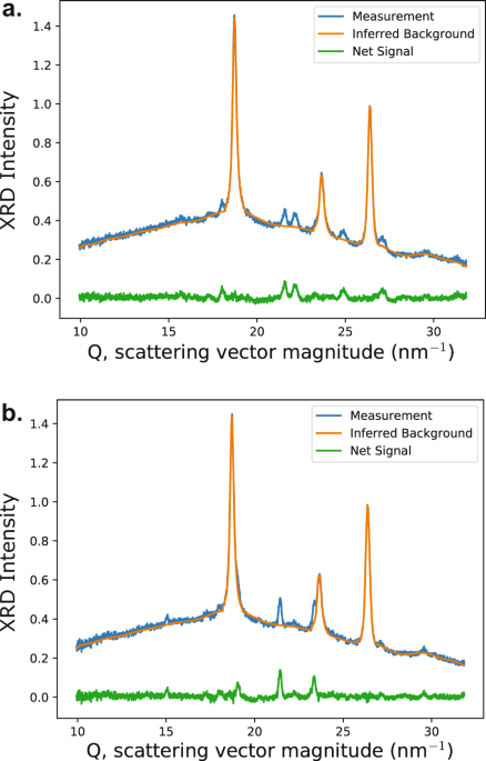
the speed and the quality of data interpretation. RESULTS X-RAY DIFFRACTION To demonstrate the performance of MCBL and illustrate some of the more subtle aspects of the model and its

deployment, we apply it to a particularly challenging XRD example in which there are multiple background sources, including a background source whose intensity is substantially higher than

the signal of interest. In this case, the strong background signal is from diffraction of the SnO2 in the substrate, introducing unwanted peaks into the dataset that are quite similar in

shape to those in the desired signal from the thin film sample. Furthermore, over a series of 186 reflection-geometry measurements on different thin film compositions, the variable density

and thickness of the thin film of interest alters the shape and intensity of the substrate signal. Provided that the set of 186 samples contains more variability in the signal of interest

than the background signal, which it does due to the variety of crystal structures in the 186 unique compositions, MCBL identifies the unique combination of background signals for each of

the 186 measured diffraction patterns. Note that we have prior knowledge that there are two distinct types of background sources: diffraction signals from the crystalline substrate and

smoothly varying signals from other sources including elastic scattering and air scattering. We inject this knowledge into the model by allowing one type of background component to have

intensity only in the vicinity of known substrate diffraction peaks (scattering vector magnitudes 18.5–19.2, 23.6–24.1, and 26.2–26.8 nm−1), while the other type of background component is

enforced to be smoothly varying. As shown in Fig. 1, the MCBL model identifies the background signal, enabling retention of the desired signal even when the Bragg peak from the sample

strongly overlaps that of the substrate. The recovery of the desired signal from the shoulder of the much more intense background signal, as exemplified by the peak near 23 nm−1 in Fig. 1b,

is uniquely enabled by the model’s ability to learn the background signal from the collection of measurements. It is also worth noting that the background models in these 2 examples are

different in slight but important ways because the total background signal is unique to each measurement, which is illustrated further in the Raman example below. RAMAN SPECTROSCOPY

Continued demonstration of MCBL proceeds with a Raman spectroscopy dataset where 2121 metal oxide samples spanning 15 pseudo-quaternary metal oxide composition spaces (5 elements including

oxygen but systematic variation of the concentrations of only the 4 metals yields dimensionality of a quaternary composition space) were measured using a rapid Raman scanning technique

described previously.19 Similar to the XRD dataset, the Raman signal from the substrate varies in intensity with sample composition, and the high sensitivity of Raman detectors to

environmental factors such as room temperature introduces additional variability in background signal. Data acquisition proceeded over a week, during which time-dependent variation in signal

levels were observed. These occur, for example, due to day to night temperature variation in the laboratory. While we expect the background to be smooth, a closed mathematical expression is

not available, making this dataset well matched to the capabilities of the MCBL model. As discussed in the Methods section, limiting each of the background signals to be smooth makes the

results relatively insensitive to the number of background sources included in the model, provided this number is at least as large as the true number of background sources. Since we expect

that several sources may be present, 16 is a convenient upper bound and is a standard value to use for datasets where more specific knowledge of the background sources is unavailable. Since

peak shapes, in particular peak widths, are more variable in Raman measurements compared to XRD measurements, and the intensity of the Raman signal of interest is often comparable to the

measurement noise, even background—Raman signals are not readily interpretable without additional information. MCBL provides such additional information, in particular the probability that

each individual data point contains signal from the sample, i.e., intensity that is not explainable by the background and noise models. For each measured signal, the algorithm produces a

probability signal that can be used to reason about the data in subsequent analysis. Since single-point outliers in the measured signals can cause single point outliers in the probablity

signal, MCBL factors in the prior knowledge that any Raman feature of interest will span several data points by smoothing the probability signal via kernel regression20 with a Gaussian

kernel of (_σ_) three data points. Thresholding the smoothed probability signals at 50% provides identification of each data point that likely contains signal from sample of interest.

Representative examples of background identification and removal are shown for three Raman measurements in Fig. 2a–c. Using MCBL with 16 background components yields background-subtracted

signals with a flat, near-zero baseline atop which the small signal peaks are far more evident than in the raw data. Since each net signal contains measurement noise, the visual

identification of peaks can be assessed in the context of this noise. The results of the probability signal analysis are shown with demarcation of each data point that likely contains signal

from the substrate. It is worth noting that researchers often apply smoothing to assist in identification of such small peaks in the signal, although the propensity for modification of the

true signal and possibilities for both false positive and false negative peak detection highlights the benefits of the identifying the background signal using a probabilistic model that

considers both the noise and the signal from the sample. Figure 2a includes examples of peaks from the sample that are notoriously difficult to identify. The peak near 480 cm−1 appears atop

of a larger peak in the background signal, and the peak near 510 cm−1 lies on a strongly sloped portion of the background signal. The intensity at the right edge of the measured signal in

Fig. 2a is increasing, so inspecting this individual pattern could not definitively identify that portion of the signal as being absent or inclusive of signal from the sample. The

probabilistic model makes this assessment, where no signal from the sample is identified in this portion of Fig. 2a. A sample peak is detected in the analogous portion of the measurement in

Fig. 2b where the partial measurement of the peak atop a sloped background would be problematic for any peak fitting (regression)-based search for sample peaks. Figure 2b also demonstrates

the importance of the multi-component aspect of the background model. While the background signal is qualitatively similar to the other samples, the quantitative differences that are

emblematic of the unique mixture of the background sources render the single-component model unable to provide a clean background-subtracted signal. The model’s detection of two peaks in the

measured signal of Fig. 2c (near 480 and 680 cm−1) is particularly impressive as even expert manual analysis may hesitate to label these features as sample peaks due to the poor

signal-to-noise ratio. Their detection in the probabilistic model is aided by the appearance of the peaks in other measurements, including that of Fig. 2a. To highlight the quality of the

net signals produced by the MCBL model, the measurement of Fig. 2c is shown in Fig. 2d along with traditional polynomial baseline modeling. The lower-order polynomial yields a net signal

where the largest peak is actually from a background source, and increasing the polynomial order to capture this feature in the background model results in removal of practically all signal

from the sample. To further illustrate the background removal and peak identification process, Fig. 3 includes a series of ten of the Raman measurements with a variety of peak locations,

shapes, and relationships to the background signal. Since the signal probability is calculated for every data point, the probability signals can be plotted in the same manner as the measured

signals, as shown in Fig. 3b. The background-subtracted samples in Fig. 3c are shown with partial transparency where the probability signal is below the 50% threshold so that the regions of

each pattern that likely contain signal from the sample are highlighted. The sharp, intense peaks in the top two patterns may be easily identified by a variety of algorithms, although

identification of many of the broader, weaker features from each sample require the excellent background identification and probabilistic reasoning of the MCBL model. PROBABILISTIC

CLASSIFICATION OF SAMPLE SIGNAL AND ENUMERATION OF BACKGROUND SOURCES Figure 2b also illustrates a subtle consequence of the model’s collective learning of the background signals,

measurement noise, and probabilities via the probabilistic framework. The rank 16 model identifies the appropriate background and consequently correctly learns the measurement noise to

identify three small peaks between 220 and 420 cm−1. The rank 1 background model is imperfect, and the collection of samples with incorrect background signals inflates the model’s estimation

of the noise level such that the resulting probability signals do not identify any of these three peaks as likely containing signal from the sample. The comprehensive probabilistic

framework enables simultaneous learning of multiple properties of the measured signals, but using a background rank smaller than the true number of background sources is deleterious not only

to background removal but also to automated detection of signals of interest. The classification of measured signals as lacking or containing a signal of interest has a variety of

applications ranging from materials discovery to characterization of the background sources. Using the rank 16 background model, 743 of the 2121 measured signals contain at least one

datapoint that is likely to contain signal of interest. Using this as the baseline classification of absence or presence of signal from the sample, the performance of lower-rank models can

be assessed via the recall (the fraction of the 743 patterns with signal that are correctly identified as having signal) and the precision (the fraction of signals with detected signal that

actually have signal). The results are summarized in Fig. 4a and demonstrate the poor performance of the rank 1 model for this classification task, which is due to a confluence of phenomena

including that noted above; non-removed background signal can be interpreted as signal of interest (false positive), and the inflated noise level in the noise model can fail to identify

small signals of interest (false negative). Increasing to rank 2 greatly improves the recall but not the precision, and increasing to rank 4 largely removes the disparity between recall and

precision. Since there is no substantial change upon increasing to rank 8, these results collectively indicate that the number of background sources is three or four. It is worth noting that

multiple components are needed to model a single background source if its signal varies in shape over the dataset, so this interpretation of rank as determine the number of sources includes

the number of unique physical phenomena that alter the shape of a background signal. The background sources can be further characterized using the wealth of information provided by the MCBL

model, such as the spatial or temporal variation in the intensity of each background source. Figure 4b includes a similar analysis for how the background-subtracted signals vary with rank.

Once again using the rank 16 results as the baseline for comparison, the difference of each background-subtracted signal is measured using both the \(\ell _1\) and root mean squared (RMS)

loss. The average per-signal loss appears to follow a power law relationship with the model rank. Each pattern contains 1023 data points, so starting at rank 4 the \(\ell _1\) value per data

point is about 1 CPS or lower, and comparison to the signals in Fig. 2 demonstrate that this is within the measurement noise, in agreement with the above observation that rank 3 or 4 is

sufficient to model the background in this dataset. Using a larger rank has no substantial influence on the resulting signals of interest. This stability in the model’s solution is an

important feature for unsupervised deployment. DISCUSSION The results above demonstrate not only successful background removal but also the generation of insightful probabilistic models for

both XRD and Raman data. While background removal is often considered a non-scientific aspect of data interpretation, consider instead the concept that the scientific merit of a chain of

analyses is only as strong as its weakest link. Artifacts injected from non-principled background subtraction are inherited by subsequent analyses and can contaminate the scientific

interpretation of the data. In general, any modification to measured data should be performed in a manner that reflects a fundamental understanding of the underlying physical processes that

give rise to the measured signals. In the present work, this understanding is incorporated with specificity through the establishment of a probability density model for the signal of

interest, yet through its parameterization the model retains generality for any measurements involving addition of non-negative sources. A desirable consequence of this principled

parameterization of the background model is that the learned parameters provide statistical characterizations of the data, which was demonstrated with analysis of the probability signals and

the identification of the number of background sources in the Raman dataset. While not discussed in the present work, after identification of the number of background sources, the

individual background signals can be analyzed to study the background sources themselves, and the activations of each of these sources in a dataset enables quantification of the variability

in each background source’s intensity. While one goal of the algorithm is the generation of background-free signals, these examples illustrate the broader application of the probabilistic

learning approach, that the optimized probabilistic model contains deep information about every component of the measured signal. A principled approach to the identification, removal and

statistical evaluation of background signals is established for any measurement type where each measured signal is a combination of non-negative contributions from multiple sources. Through

design of a parameterized probability density function for the measured intensities of a signal of interest, a probabilistic framework is established for unsupervised learning of background

signals, in particular when there are multiple sources of background whose contributions to the measured signal vary among the set of measurements. In addition to unsupervised operation, the

model provides a variety of methods for incorporating prior knowledge, which is demonstrated with an example XRD dataset in which the crystalline substrate produces more intense diffraction

patterns than the sample of interest. The probability signals, which indicate where the signal of interest is likely present, are demonstrated using a Raman dataset in which the ~4

background sources are identified and modeled for each measurement, providing signals for further analysis that contain negligible contributions from the background. The probability signals

and other parameters can be employed by subsequent reasoning and learning algorithms, making the algorithm a foundational advancement in the automation of data interpretation. METHODS MCBL

MODEL In a dataset with _N_ signals that were measured on a variety of samples, each signal _S__i_ is modeled as the sum of the signal _P__i_ from the sample, which typically involves a

series of peaks, and the total background signal _B__i_. For each data point _j_ in measurement _i_, $$S_{i,j} = P_{i,j} + B_{i,j}.$$ (1) Since in general _B__i_ is composed of a unique

mixture of _K_ background signals, the background patterns and sample-specific weights are determined using a matrix factorization (MF) approach. The MF construction of the background model

involves the matrix _V_, containing the collection of _K_ signals from the background sources, and the matrix _U_, containing the amount of each background signal in each measured signal.

The matrix product _UV_ is thus the collection of total background signals for each measurement: _B_ ≈ _UV_. To create a model that does not require measurement of each background signal,

which is typically not possible, the matrices _U_ and _V_ are learned from the measured spectra by considering the MF problem $$S \approx UV.$$ (2) In traditional implementations of matrix

factorization, the residuals of the model, _R_ = _S_ − _UV_, are minimized with respect to \(\ell _2\) or similar loss metric. However, given that _UV_ is the background model, _R_ contains

_P_, the signals of interest. In spectroscopic data, _P_ is positive and can be large. Critically, large deviations are penalized heavily by traditional loss functions like \(\ell _2\).

Therefore, this problem requires a novel approach to solving the matrix factorization problem, which allows for large deviations from the background model _UV_ where signals of interest are

present. If the signal of interest includes a peak (non-background signal) at the _j_th data point in measurement _i_, then _R__i_,_j_ will be large and positive. While _R__i_,_j_ should be

near zero for data points containing only background signal, the measurements _S_ and thus the residuals _R_ contain measurement noise. As a result, the distribution of _R__i_,_j_ values

will be different when the signal of interest is absent or present. When absent, the measurement noise is typically well modeled by a Gaussian distribution, \({\cal{N}}_{\mu ,\sigma }\).

When present, the large residual intensities (peaks) are modeled by an exponential distribution, which when combined with the Gaussian distribution for noise yields the exponentially

modified Gaussian (EMG) distribution: $${\mathrm{EMG}}_{\mu ,\sigma ,\lambda }(R_{ij}) = \frac{\lambda }{2}e^{\frac{\lambda }{2}(2\mu + \lambda \sigma ^2 - 2R_{ij})}\,{\mathrm{erfc}}\,\left(

{\frac{{\mu + \lambda \sigma ^2 - R_{ij}}}{{\sqrt 2 \sigma }}} \right),$$ (3) where erfc is the complementary error function, _λ_ is the rate parameter of the exponential random variable,

and _μ_ and _σ_ are the location and scale parameters of the Gaussian random variable, respectively. This distribution was previously used in biology,21 psychology,22 and finance.23

Furthermore, the values _λ_, _μ_, and _σ_ can vary along the measurement axis to increase the flexibility of the model, if required. In the present work we consider only a single _σ_ and _λ_

for a given dataset and fix the mean _μ_ of the Gaussian noise to zero. Since \({\cal{N}}_{\mu ,\sigma }\) and the EMG distribution of Eq. (3) describe the distribution of residual

intensities when the signal of interest is absent and present, respectively, a general expression for the distribution of residual intensities is their mixture: $$\begin{array}{*{20}{l}}

{{\mathrm{EMGM}}_{\mu ,\sigma ,\lambda ,Z_{ij}}(R_{ij}): = (1 - Z_{ij}){\cal{N}}_{\mu ,\sigma }(R_{ij}) + Z_{ij}\,{\mathrm{EMG}}_{\mu ,\sigma ,\lambda }(R_{ij}),} \hfill \end{array}$$ (4)

where _Z__ij_ indicates whether signal of interest is absent (_Z__ij_ = 0) or present (_Z__ij_ = 1) in the residual _R__ij_. Optimization of the matrix factorization model Eq. (2)

corresponds to finding the background patterns, weights and distribution parameters such that the likelihood, corresponding to the product of Eq. (4) for all data points, is maximized. This

enables _U_, _V_, _Z_, _λ_, _μ,_ and _σ_ to be learned concomitantly. A standard procedure in machine learning is to regularize optimization problems to make them well posed. In particular,

to encourage the algorithm to find solutions with a small noise variance, we added a half normal prior on _σ_ to regularize the optimization with respect to the parameter. The prior

distribution has a variance \(\sigma _0^2\) which can be used to control the strength of the regularization. This is necessary for the XRD dataset, since it does not include any substrate

measurements. Therefore, we used \(\sigma _0^2 = 0.01\) for the XRD dataset. Because the exact optimization of the binary variables _Z__i_,_j_ is computationally intractable, we employ an

expectation-maximization algorithm.24,25 Instead of inferring _Z__i_,_j_ directly, the algorithm computes the expected value \({\mathbb{E}}(Z_{ij})\), which is a continuous variable in the

interval [0, 1]. From the equality $${\mathbb{E}}[Z_{ij}]={\mathbb{P}}(Z_{ij} = 1),$$ (5) we also obtain the probability that the measured data point _S__i_,_j_ contains non-background

signal. The algorithm for solving this implementation of probabilistic matrix factorization is described in ref. 26. This approach to background identification enables unsupervised learning

of the background model after choosing the value of a single parameter, the rank _K_ of _V_, which corresponds to the number of background sources. While unsupervised methods for determining

an appropriate value of _K_ can be deployed,27 we instead further constrain the matrix factorization model such that the results are relatively insensitive to _K_. This enables users to

choose an upper bound for _K_ and retain unsupervised operation. The constraints to the matrix factorization also enable semi-supervised operation, which enables both injection of prior

knowledge of the background sources and deployment in data-starved situations where there are not enough examples of the background signals for the unsupervised model to robustly learn them.

The constraints are implemented by defining kernel functions for each component of _V_. The most commonly used kernel is the squared exponential (SE) kernel, which enforces smoothness of

each background signal. For example, the background model for the Raman data was obtained by using the SE kernel for all background components. Further, if the underlying physics of a given

background signal give rise to a functional form or another physics-based constraint, this too can be used to constrain components in _V_. In fact, for the XRD dataset, the SE kernel was

only used for two background signals. The other two background signals were constrained based on prior knowledge of the background signal from the crystalline substrate; the intensity of

these background signals was constrained to zero except for the regions indicated above in the X-ray diffraction section. This is done with a simple projection: All values outside of the

allowed ranges are set to zero in every gradient step of the optimization algorithm. Despite there only being one crystalline substrate, we used two vectors to express its signature to

accommodate for any variations in this background signal over the set of measurements. LIBRARY SYNTHESIS The pseudo-ternary metal oxide composition gradient was fabricated using reactive

direct current magnetron co-sputtering of Cu, Ca, and V metal targets in a non-confocal geometry onto a 100 mm diameter × 2.2 mm thick soda lime glass substrate with FTO coating (Tec15,

Hartford Glass Company) in a sputter deposition system (Kurt J. Lesker, PVD75) at 10−5 Pa base pressure. The partial pressures of the deposition atmosphere containing inert sputtering gas Ar

and reactive gas O2 were 0.072 Pa and 0.008 Pa respectively. Deposition proceeded without active substrate heating, with the source powers set to 150 W, 11 W, and 95 W for the V, Cu, and Ca

sources respectively. Deposition time per source was varied in order to achieve a total film thickness of 200 nm. The as-deposited composition library was annealed in a Thermo Scientific

box oven in flowing air, with a 2 h ramp and 3 h soak at 550 °C, followed by passive cooling. The 2121 samples forming the 15 pseudo-quaternary space composition library were deposited via

inkjet printing onto 100 × 150 × 1.0 mm fluorine-doped tin oxide (FTO) coated boro-aluminosilicate glass (Corning Eagle XG Glass). The array of samples containing Mn, Fe, Ni, Cu, Co, and Zn

was synthesized as a discrete library with 10 atom% composition steps in each element, using a print resolution of 2880 × 1440 dpi, as described previously.28 Elemental precursor inks were

prepared by mixing 3.33 mmoles of each metal precursor with 20 mL of stock solution. The stock solution of 500 mL 200 proof ethanol (Koptec), 16 mL glacial acetic acid (T.J. Baker, Inc.), 8 

mL concentrated HNO3 (EMD), and 13 g Pluronic F127 (Aldrich) was prepared beforehand. The metal precursors Mn(NO3)2 4⋅H2O (0.88 g, 99.8%, Alfa Aesar), Fe(NO3)3 9⋅H2O (1.43 g, 99.95%, Sigma

Aldrich), Co(NO3)2 6⋅H2O (0.93 g, 98%, Sigma Aldrich), Ni(NO3)2 6⋅H2O (1.09 g, 98.5%, Sigma Aldrich), Cu(NO3)2 3⋅H2O (0.83 g 99–104%, Sigma Aldrich), and Zn(NO3)2 6⋅H2O (1.00 g 98%, Sigma

Aldrich) were used as-received from the distributor. After inkjet printing, the inks were dried and converted to metal oxides by calcination in 0.395 atm O2 at 450 °C for 10 h, followed by

0.395 atm O2 at 750 °C for 10 h. X-RAY DIFFRACTION XRD was performed on the pseudo-ternary metal oxide composition gradient using a Bruker DISCOVER D8 diffractometer, with a Bruker IμS

source emitting Cu K_α_ radiation. Using a 0.5 mm collimator, the measurement area was approximately 0.5 mm × 1 mm. Within this measurement area the composition is uniform to with about 1 

at.%. Measurements were taken on an array of 186 evenly spaced positions across the continuous composition library. Two-dimensional diffraction images taken by the VÅNTEC-500 detector were

integrated into one-dimensional patterns using DIFFRAC.SUITETM EVA software. RAMAN SPECTROSCOPY The 15 pseudo-quaternary composition space metal oxide sample library, was characterized using

a Renishaw inVia Reflex Micro Raman spectrometer with Wire 4.1 software as described previously.19 The instrument’s laser wavelength was 532 nm, and the diffraction grating resolution 2400

lines mm−1 (visible). Spectra were taken over the range 67–1339.9 cm−1 using a ×20 objective. The Renishaw StreamlineTM mapping system was used to automate spectral image collection in which

a cylindrical lens-expanded 26 × 2 μm laser line was rastered over the measurement area. Spectra were acquired at 65 μm spatial resolution and 0.75 s exposure time. DATA AVAILABILITY The

datasets analyzed during the current study are available in the Caltech Data repository: XRD at https://doi.org/10.22002/D1.1178, https://data.caltech.edu/records/1178 and Raman at

https://doi.org/10.22002/D1.1179, https://data.caltech.edu/records/1179. CODE AVAILABILITY The codes pertaining to the current study will be available at

http://www.cs.cornell.edu/gomes/udiscoverit/. REFERENCES * Alberi, K. et al. The 2019 materials by design roadmap. _J. Phys. D_ 52, 013001 (2019). Article  Google Scholar  * Aspuru-Guzik, P.

K. A. Alán. Report of the Clean Energy Materials Innovation Challenge Expert Workshop January 2018, Mission Innovation

http://mission-innovation.net/wp-content/uploads/2018/01/Mission-Innovation-IC6-Report-Materials-Acceleration-Platform-Jan-2018.pdf. * Tabor, D. P. et al. Accelerating the discovery of

materials for clean energy in the era of smart automation. _Nat. Rev. Mater._ 3, 5 (2018). Article  CAS  Google Scholar  * Laue, M. Über die Interferenzerscheinungen an planparallelen

Platten. _Ann. der Phys._ 318, 163–181 (1904). Article  Google Scholar  * Seah, M. P. The quantitative analysis of surfaces by xps: a review. _Surf. Interface Anal._ 2, 222–239 (1980).

Article  CAS  Google Scholar  * Sonneveld, E. J. & Visser, J. W. Automatic collection of powder data from photographs. _J Appl. Crystallograph_. 8, 1–7 (1975). * Tougaard, S. Algorithm

for automatic X-ray photoelectron spectroscopy data processing and x-ray photoelectron spectroscopy imaging. _J. Vac. Sci. Technol._ 23, 741–745 (2005). Article  CAS  Google Scholar  *

Hattrick-Simpers, J. R., Gregoire, J. M. & Kusne, A. G. Perspective: composition–structure–property mapping in high-throughput experiments: turning data into knowledge. _APL Mater._ 4,

053211 (2016). Article  Google Scholar  * Stein, H. S., Jiao, S. & Ludwig, A. Expediting combinatorial data set analysis by combining human and algorithmic analysis. _ACS Comb. Sci._ 19,

1–8 (2017). Article  CAS  Google Scholar  * Tessier, F. & Kawrakow, I. Calculation of the electron–electron bremsstrahlung cross-section in the field of atomic electrons. _Nucl. Instr.

Meth. Phys. Res. B_ 266, 625–634 (2008). * Kramers, H. A. Xciii. on the theory of x-ray absorption and of the continuous x-ray spectrum. _Lond. Edinb. Dublin Philos. Mag. J. Sci._ 46,

836–871 (1923). Article  CAS  Google Scholar  * Davies, H., Bethe, H. A. & Maximon, L. C. Theory of Bremsstrahlung and pair production. II. Integral cross section for pair production.

_Phys. Rev._ 93, 788–795 (1954). Article  CAS  Google Scholar  * Bethe, H. A. & Maximon, L. C. Theory of Bremsstrahlung and pair production. I. Differential cross section. _Phys. Rev._

93, 768–784 (1954). Article  CAS  Google Scholar  * Tougaard, S. & Jorgensen, B. Inelastic background intensities in XPS spectra. _Surface Sci_. 143, 482–494 (1984). * Zhao, J., Lui, H.,

McLean, D. I. & Zeng, H. Automated autofluorescence background subtraction algorithm for biomedical raman spectroscopy. _Appl. Spectrosc._ 61, 1225–1232 (2007). Article  CAS  Google

Scholar  * Markus, G., Konstantinos, N., Frank, P., Christian, M. & Andreas, O. Multivariate characterization of a continuous soot monitoring system based on Raman spectroscopy. _Aerosal

Sci. Technol_. 49, 997–1008 (2015). * Li, Z., Ludwig, A., Savan, A., Springer, H. & Raabe, D. Combinatorial metallurgical synthesis and processing of high-entropy alloys. _J. Mater.

Res._ 33, 3156–3169 (2018). Article  CAS  Google Scholar  * Zhao, J. Combinatorial approaches as effective tools in the study of phase diagrams and composition–structure–property

relationships. _Prog. Mater. Sci._ 51, 557–631 (2006). Article  Google Scholar  * Newhouse, P. F. et al. Solar fuel photoanodes prepared by inkjet printing of copper vanadates. _J. Mater.

Chem. A_ 4, 7483–7494 (2016). Article  CAS  Google Scholar  * Wand, M. & Jones, M. Kernel Smoothing. New York: Chapman and Hall/CRC (1995). * Golubev, A. Exponentially modified gaussian

(emg) relevance to distributions related to cell proliferation and differentiation. _J. Theor. Biol._ 262, 257–266 (2010). Article  CAS  Google Scholar  * Palmer, E. M., Horowitz, T. S.,

Torralba, A. & Wolfe, J. M. What are the shapes of response time distributions in visual search? _J. Exp. Psychol. Hum. Percept. Perform._ 37, 58–71 (2011). Article  Google Scholar  *

Carr, P., Madan, D. & Smith, H. R. Saddle point methods for option pricing. _J. Comput. Financ._ 13, 49–61 (2009). Article  Google Scholar  * Dempster, A. P., Laird, N. M. & Rubin,

D. B. Maximum likelihood from incomplete data via the em algorithm. _J. R. Stat. Soc. Ser. B_ 39, 1–38 (1977). Google Scholar  * Neal, R. M. & Hinton, G. E. _Learning in Graphical

Models._ (MIT Press, Cambridge, 1999). Google Scholar  * Ament, S., Gregoire, J. & Gomes, C. Exponentially-modified Gaussian mixture model: applications in spectroscopy. Preprint at

arXiv:1902.05601 (2019). * Neal, R. M. Markov chain sampling methods for dirichlet process mixture models. _J. Comput. Graph. Stat._ 9, 249–265 (2000). Google Scholar  * Haber, J. A. et al.

Discovering ce-rich oxygen evolution catalysts, from high throughput screening to water electrolysis. _Energy Environ. Sci._ 7, 682–688 (2014). Article  CAS  Google Scholar  Download

references ACKNOWLEDGEMENTS The development of the MCBL algorithm, inkjet printing synthesis, and Raman measurements were supported by a an Accelerated Materials Design and Discovery grant

from the Toyota Research Institute. Initial design of the algorithm and data procurement were supported by the NSF Expedition award for Computational Sustainability CCF-1522054 and by Army

Research Office (ARO) award W911-NF-14-1-0498. The implementation of the algorithm for automated, unsupervised operation was supported by MURI/AFOSR grant FA9550. Compute infrastructure was

provided by NSF award CNS-0832782 and by ARO DURIP award W911NF-17-1-0187. The sputter deposition and XRD measurements were supported through the Office of Science of the U.S. Department of

Energy under Award No. DE-SC0004993. The authors thank Edwin Soedarmadji for assistance with data management. AUTHOR INFORMATION AUTHORS AND AFFILIATIONS * Department of Computer Science,

Cornell University, Ithaca, NY, 14850, USA Sebastian E. Ament & Carla P. Gomes * Joint Center for Artificial Photosynthesis, California Institute of Technology, Pasadena, CA, 91125, USA

Helge S. Stein, Dan Guevarra, Lan Zhou, Joel A. Haber, David A. Boyd, Mitsutaro Umehara & John M. Gregoire * Future Mobility Research Department, Toyota Research Institute of North

America, Ann Arbor, MI, 48105, USA Mitsutaro Umehara Authors * Sebastian E. Ament View author publications You can also search for this author inPubMed Google Scholar * Helge S. Stein View

author publications You can also search for this author inPubMed Google Scholar * Dan Guevarra View author publications You can also search for this author inPubMed Google Scholar * Lan Zhou

View author publications You can also search for this author inPubMed Google Scholar * Joel A. Haber View author publications You can also search for this author inPubMed Google Scholar *

David A. Boyd View author publications You can also search for this author inPubMed Google Scholar * Mitsutaro Umehara View author publications You can also search for this author inPubMed 

Google Scholar * John M. Gregoire View author publications You can also search for this author inPubMed Google Scholar * Carla P. Gomes View author publications You can also search for this

author inPubMed Google Scholar CONTRIBUTIONS C.G. and J.G. identified the problem to be solved. S.A. and C.G. conceptualized the model. S.A. developed the mathematical framework, designed

the algorithm, and implemented it. J.G., H.S. and D.G. inspected results. S.A., D.G. and J.G. created visualizations of the results. L.Z. performed materials synthesis and data acquisition

for XRD data. J.H. synthesized materials for Raman measurements. D.B. and M.U. acquired and provided the Raman data. S.A., J.G., C.G., H.S. and D.G. wrote the paper. CORRESPONDING AUTHORS

Correspondence to John M. Gregoire or Carla P. Gomes. ETHICS DECLARATIONS COMPETING INTERESTS The authors declare no competing interests. ADDITIONAL INFORMATION PUBLISHER’S NOTE: Springer

Nature remains neutral with regard to jurisdictional claims in published maps and institutional affiliations. RIGHTS AND PERMISSIONS OPEN ACCESS This article is licensed under a Creative

Commons Attribution 4.0 International License, which permits use, sharing, adaptation, distribution and reproduction in any medium or format, as long as you give appropriate credit to the

original author(s) and the source, provide a link to the Creative Commons license, and indicate if changes were made. The images or other third party material in this article are included in

the article’s Creative Commons license, unless indicated otherwise in a credit line to the material. If material is not included in the article’s Creative Commons license and your intended

use is not permitted by statutory regulation or exceeds the permitted use, you will need to obtain permission directly from the copyright holder. To view a copy of this license, visit

http://creativecommons.org/licenses/by/4.0/. Reprints and permissions ABOUT THIS ARTICLE CITE THIS ARTICLE Ament, S.E., Stein, H.S., Guevarra, D. _et al._ Multi-component background learning

automates signal detection for spectroscopic data. _npj Comput Mater_ 5, 77 (2019). https://doi.org/10.1038/s41524-019-0213-0 Download citation * Received: 18 February 2019 * Accepted: 26

June 2019 * Published: 19 July 2019 * DOI: https://doi.org/10.1038/s41524-019-0213-0 SHARE THIS ARTICLE Anyone you share the following link with will be able to read this content: Get

shareable link Sorry, a shareable link is not currently available for this article. Copy to clipboard Provided by the Springer Nature SharedIt content-sharing initiative