Overcoming bias in estimating epidemiological parameters with realistic history-dependent disease spread dynamics

ABSTRACT Epidemiological parameters such as the reproduction number, latent period, and infectious period provide crucial information about the spread of infectious diseases and directly

inform intervention strategies. These parameters have generally been estimated by mathematical models that involve an unrealistic assumption of history-independent dynamics for simplicity.

This assumes that the chance of becoming infectious during the latent period or recovering during the infectious period remains constant, whereas in reality, these chances vary over time.

Here, we find that conventional approaches with this assumption cause serious bias in epidemiological parameter estimation. To address this bias, we developed a Bayesian inference method by

adopting more realistic history-dependent disease dynamics. Our method more accurately and precisely estimates the reproduction number than the conventional approaches solely from confirmed

cases data, which are easy to obtain through testing. It also revealed how the infectious period distribution changed throughout the COVID-19 pandemic during 2020 in South Korea. We also

provide a user-friendly package, IONISE, that automates this method. SIMILAR CONTENT BEING VIEWED BY OTHERS EVALUATING A NOVEL REPRODUCTION NUMBER ESTIMATION METHOD: A COMPARATIVE ANALYSIS

Article Open access 13 February 2025 IMPROVED ESTIMATION OF THE EFFECTIVE REPRODUCTION NUMBER WITH HETEROGENEOUS TRANSMISSION RATES AND REPORTING DELAYS Article Open access 15 November 2024

INFERRING THE SPREAD OF COVID-19: THE ROLE OF TIME-VARYING REPORTING RATE IN EPIDEMIOLOGICAL MODELLING Article Open access 24 June 2022 INTRODUCTION Viruses, outnumbering all other life

forms, are omnipresent in nature and exhibit parasitic characteristics by depending on host cells for replication1,2. Some viruses cause severe infectious diseases in humans and animals,

with substantial medical, social, and economic impacts. To mitigate these impacts, understanding disease spread dynamics is crucial as it allows for the development of effective control

measures, including vaccination strategies3. The spread dynamics of an infectious disease can be described by various epidemiological parameters. Among them, the most important parameter is

the reproduction number (\({{\mathscr{R}}}\)), which represents the average number of secondary infections caused by an infected individual throughout the infectious period. Recently, the

COVID-19 pandemic has highlighted the importance of estimating \({{\mathscr{R}}}\) to evaluate the severity of the outbreak and the effectiveness of interventions4. For the estimation of

\({{\mathscr{R}}}\), mathematical models have been widely employed5,6,7. These models typically divide the population into distinct compartments and incorporate assumptions about the

transition rates between the compartments. Two crucial time intervals within these models are the latent and infectious periods. The latent period is the time from exposure to the onset of

infectiousness, and the infectious period is the time from the onset of infectiousness to the loss of infectiousness due to recovery8. The latent and infectious periods are often assumed to

follow exponential distributions in these models because this assumption facilitates model analysis and inference using simple ordinary differential equations (ODEs). However, exponentially

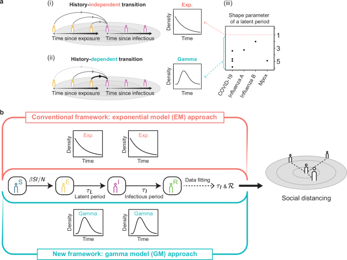
distributed latent and infectious periods do not align with the epidemiological reality of most infections9. Specifically, it implies history-independent transitions, i.e., the chance of

leaving the exposed or infectious compartment remains unchanged regardless of time since exposure or being infectious, respectively (Fig. 1a(i)). Thus, relying on this unrealistic assumption

can introduce systematic bias into the models and potentially lead to erroneous policy recommendations. An alternative approach is to consider history-dependent transitions between

compartments. That is, the chances of leaving the compartments are initially low but increase as the time since exposure and being infectious increase (Fig. 1a(ii)). The history-dependent

transitions can be implied by gamma distributed latent and infectious periods. Indeed, the latent periods of various infectious diseases, such as COVID-19, influenza, and Mpox, follow gamma

distributions, indicated by shape parameters greater than one (Fig. 1a(iii))10,11,12,13,14,15,16. Similarly, the infectious periods of various diseases also follow gamma distributions9. To

incorporate realistic gamma distributions for latent and infectious periods, a linear chain trick has frequently been used9,17,18,19. This involves adding subcompartments with the same

transition rates. Then, latent and infectious periods follow Erlang distributions (i.e., gamma distributions with integer shape parameters) because the sum of independent and identically

distributed exponential random variables follows a gamma distribution. However, adding artificial subcompartments makes the model complex. To avoid this, discrete-time compartment models or

a system of integro-differential equations have been employed. In discrete-time compartment models, sojourn times in compartments are sampled from delay distributions to incorporate

realistic latent and infectious periods20,21,22. In a system of integro-differential equations, realistic latent and infectious period distributions are incorporated with their probability

density functions, which directly take the history-dependent transition into account23,24,25. While these approaches successfully incorporate the realistic distributions of latent and

infectious periods, they can estimate \({{\mathscr{R}}}\) only when the distributions of latent and infectious periods are known. However, unlike latent periods, which are inherent

characteristics of disease dynamics, infectious periods are rarely known. Furthermore, previously calculated infectious periods cannot be used due to their potential variation across time,

regions, and non-pharmaceutical intervention measures26,27,28,29. For instance, the infectious period calculated using data from China shortened significantly from 5.5 days to 1.5 days over

time30. In this work, we address this challenge by developing a Bayesian Markov Chain Monte Carlo (MCMC) method that estimates \({{\mathscr{R}}}\) solely based on easy-to-obtain data (i.e.,

cumulative confirmed cases) while incorporating realistic distributions for latent and infectious periods. Specifically, our method estimates \({{\mathscr{R}}}\) by fitting observed data and

simulated data from delay differential equations (DDEs) that describe the dynamics of the non-Markovian compartmental model with gamma distributed latent and infectious periods, indicating

history-dependent transitions between compartments (Fig. 1a(ii)). Compared to the conventional ODE-based method, which assumes unrealistic history-independent transitions (Fig. 1a(i)), our

method provides a much more accurate estimation of \({{\mathscr{R}}}\). It matches the \({{\mathscr{R}}}\) value separately estimated with intensive contact tracing, although our method

estimates it using only easy-to-obtain cumulative confirmed case. The estimated \({{\mathscr{R}}}\) values remain robust even when the initial number of exposed individuals is uncertain,

which commonly arises during the course of disease spread. Importantly, our method estimates the infectious period distribution more accurately than the conventional method and reveals how

the infectious period distribution changed throughout the COVID-19 pandemic during 2020 in South Korea, providing valuable information on the evolution of intervention effectiveness over

time. Furthermore, we provide a user-friendly computational package implementing our method, called IONISE (Inference Of Non-markovIan SEir model) (https://github.com/mathbiomed/IONISE)31.

Using IONISE, we apply our method to models with more general (e.g., lognormal and Weibull) distributions and complex disease dynamics (e.g., vaccination, variants, and unreported cases),

demonstrating the versatility and scalability of our method. RESULTS DEVELOPMENT OF AN SEIR MODEL INCORPORATING REALISTIC GAMMA DISTRIBUTIONS OF LATENT AND INFECTIOUS PERIODS Among various

epidemiological compartmental models that can incorporate the latent and infectious periods of infectious diseases, an SEIR model is one of the most widely- employed models32,33,34,35. It

consists of four compartments: individuals susceptible to infection (_S_); individuals exposed to infection (_E_), i.e., individuals who have been infected but do not exhibit infectiousness;

individuals who exhibit infectiousness (_I_); and individuals who have been removed from the system (_R_), i.e., no longer exhibit infectiousness due to, for example, recovery or isolation.

The latent period is the time from exposure to infectious pathogens to becoming infectious (i.e., from _E_ to _I_), and the infectious period is the time from becoming infectious to no

longer being infectious (i.e., from _I_ to _R_). See Methods for a detailed interpretation of the infectious period in this work. To estimate the epidemiological parameters of the SEIR

model, we fit the model with observed cumulative confirmed cases using a Bayesian MCMC method based on the Poisson likelihood function (see Supplementary Note 4). This allows the estimation

of transmission rate (\(\beta\)), latent period (\({\tau }_{L}\)), infectious period (\({\tau }_{I}\)), and \({{\mathscr{R}}}\). The \({{\mathscr{R}}}\) value is given by \(\beta \times {\mu

}_{{\tau }_{I}}\) where \({\mu }_{{\tau }_{I}}\) is the mean of \({\tau }_{I}\). This conventional approach relies on the assumption that \({\tau }_{L}\) and \({\tau }_{I}\) are

exponentially distributed since the ODEs are the law of large numbers limits of the stochastic SEIR model with the exponentially distributed \({\tau }_{L}\) and \({\tau }_{I}\)36. Thus, we

refer to this approach as the exponential model (EM) approach (Fig. 1b, top). The exponentially distributed latent period implies history-independent transitions between compartments (Fig. 

1a(i)). In other words, the chance of becoming infectious for an exposed individual remains unchanged even when the time since exposure increases. However, this assumption of the

exponentially distributed latent period is unrealistic because, in reality, the chance of becoming infectious after exposure increases as time since exposure increases (i.e.,

history-dependent transition) (Fig. 1a(ii)). Thus, it is preferable to assume that the latent period follows a gamma distribution, which implies history-dependent transitions37. Indeed, the

latent periods of various diseases follow gamma distributions whose shape parameter is greater than one (Fig. 1a(iii)). Similarly, the infectious periods of various diseases also follow

gamma distributions9. To adopt the more realistic assumption of gamma-distributed latent and infectious periods, we developed a new framework, called the gamma model (GM) approach (Fig. 1b,

bottom). First, we formulated the DDEs that describe the SEIR model with gamma-distributed latent and infectious periods (see Methods and Supplementary Note 1 for details). Note that this is

distinguished from previous works using the fixed time delay rather than distributed time delay38,39,40. Then, we fit observed data using simulated data from the DDEs and estimate

\(\beta\), \({\tau }_{I}\), and \({{\mathscr{R}}}\). For parameter estimation, we used the Bayesian MCMC method as we did in the EM approach. To facilitate the use of this approach, we

developed a user-friendly computational package, IONISE31, that implements the GM approach, along with a step-by-step manual (see Supplementary Note 2). DURING THE INITIAL PHASE OF DISEASE

SPREAD, THE GM APPROACH ACCURATELY ESTIMATES THE INFECTIOUS PERIOD DISTRIBUTION AND REPRODUCTION NUMBER To compare the estimation results based on the EM and GM approaches, we used the

cumulative confirmed COVID-19 cases data in Seoul, South Korea, from 20 January 2020 to 25 November 2020 (Fig. 2). Specifically, we examined three periods where noticeable increases of cases

were observed: the initial phase (20 January 2020 to 3 March 2020), the second wave (1 August 2020 to 19 August 2020), and the third wave (1 November 2020 to 25 November 2020). The

increases in infections during the initial phase, second wave, and third wave were caused by early disease transmission, a mass gathering on Korean Liberation Day, and a reduced social

distancing measure, respectively. During the initial phase (Fig. 3a), contact tracing was intensively conducted to minimize under-reporting of cases. We have used this to estimate the

empirical reproduction number, which represents the mean of secondary infections across all primary cases during a specified time period, following a previous study41 (see Supplementary Note

 3 for details). These data enable the calculation of the average \({{\mathscr{R}}}\) value, which is 2.7 (Fig. 3b). To assess how accurately the EM and GM approaches estimate

\({{\mathscr{R}}}\) value and \({\tau }_{I}\) distribution, we fit the data using the two approaches and estimated \(\beta\) and \({\tau }_{I}\). During the estimation, \({\tau }_{L}\) was

set to be known because it can be separately estimated from previously reported data16. Specifically, as \({\tau }_{L} \sim \Gamma (4.06,\;1.35)\) is previously reported, we used for the GM

approach (Fig. 3a, inset). On the other hand, as the gamma distribution cannot be incorporated in the EM approach, we used \({\tau }_{L} \sim {{\rm{Exp}}}({\left(4.06\times

1.35\right)}^{-1})\), which has the same mean (=5.5 days) to the gamma distribution, as done in previous studies42,43. For the initial values of the compartments _S_, _E_, _I_, and _R_, we

set them to represent that the entire population of Seoul (\(N\approx {10}^{7}\)) is susceptible except for one infectious individual, consistent with the data. While both approaches fit

well to observed confirmed cases (Fig. 3a), the estimated parameters were different. The EM approach resulted in smaller estimates of \(\beta\) and larger estimates of \({\mu }_{{\tau

}_{I}}\) and \({{\mathscr{R}}}\), compared with the GM approach (Fig. 3c). In particular, the \({\mu }_{{\tau }_{I}}\) value estimated by the GM approach was 5.3 days (95% confidence

interval, 4.6–6.4). This estimate closely aligns with the mean \({\tau }_{I}\) value of 5.4 days (4.6–6.3) reported in a previous study that also analyzes the same phase and region44 while

the EM approach provided an unrealistically high \({\mu }_{{\tau }_{I}}\) value of 14.4 days (11.8–17.2). Notably, the \({{\mathscr{R}}}\) value estimated by the GM approach, but not the EM

approach, was similar to the \({{\mathscr{R}}}\) value calculated from the contact tracing data, 2.7 (Fig. 3c, right, dashed line). This significant difference in the estimations between the

EM and GM approaches implies that assuming exponential distributions for the latent and infectious periods can lead to considerable bias. This overestimation of the reproduction number is

consistent with previously reported results where assuming exponential distributions led to overestimated reproduction numbers9,45. Furthermore, the GM approach can estimate the distribution

of \({\tau }_{I}\) with a more realistic shape compared to the EM approach. The estimated distribution is noticeably different from an exponential distribution (i.e., shape parameter \(\gg

1\)) (Fig. 3d), indicating that the distribution cannot be captured by the EM approach. The distribution of \({\tau }_{I}\) can provide valuable information for understanding the dynamics of

infectious diseases, guiding public health responses, and developing effective strategies to control and mitigate their impact on populations46,47. For example, since the density is nearly

zero after 10 days, it could be used to set the length of the isolation period to prevent the spread of disease. To systematically analyze the results obtained from the real-world data, we

performed data fitting on simulation data generated with various \({{\mathscr{R}}}\) values (1, 2, and 4) (Fig. 3e). For data generation, we used \({\tau }_{L} \sim \Gamma

({\mathrm{4.06,\;1.35}})\), \({\tau }_{I} \sim \Gamma ({\mathrm{30,\;0.2}})\), and initial conditions that mimic the initial phase (Fig. 3a). We estimated the parameters when \({\tau }_{L}\)

is known as we did with the real-world data (Fig. 3a–d). While the GM approach yielded accurate estimates, the EM approach underestimated \(\beta\) and considerably overestimated both

\({\mu}_{{\tau }_{I}}\) and \({{\mathscr{R}}}\) (Fig. 3f), consistent with the estimation results obtained with the real-world data (Fig. 3c). Importantly, the GM approach accurately

estimated the distribution of \({\tau }_{I}\) (Fig. 3g). In particular, the mean of distributions with posterior samples (Fig. 3g, blue line) was close to the true distribution of \({\tau

}_{I}\) used to generate the data (Fig. 3g, black line). The true distribution was contained in the 95% confidence interval of estimated distributions of \({\tau }_{I}\) (Fig. 3g, gray

region). We investigated whether the overestimations of \({{\mathscr{R}}}\) by the EM approach could be resolved with additional information, specifically knowing the infectious period

\({\tau }_{I}\) (Fig. 3h). With this additional information, the EM approach provided accurate estimates of \(\beta\) and \({{\mathscr{R}}}\), similar to the GM approach (Fig. 3i). However,

it is rare to have access to information on \({\tau }_{I}\) as it can vary across time, regions, and non-pharmaceutical intervention measures unlike \({\tau }_{L}\)26,27,28,29,30, which can

be separately calculated from past contact tracing data. DURING THE MIDDLE OF THE DISEASE SPREAD, \({{\MATHSCR{R}}}\) ESTIMATION WITH THE GM APPROACH IS ROBUST TO THE INITIAL NUMBER OF

EXPOSED INDIVIDUALS At the beginning of the initial phase, the entire population is susceptible except for one infectious individual. However, during the middle phase of disease spread, the

numbers of exposed individuals (\(E(0)\)) and infectious individuals (\(I(0)\)) at the beginning need to be specified. To compare the performance of the EM and GM approaches for estimating

epidemiological parameters during the middle of the disease spread, we applied them to the second wave data from Seoul, South Korea (1 August 2020 to 19 August 2020) (Fig. 2). In these data,

\(I\left(0\right)=25\) can be determined by the number of individuals who are symptomatic but not confirmed in the contact tracing data. \(R\left(0\right)=1607\) can also be determined by

the number of cumulative confirmed cases at the beginning of the wave. However, determining \(E(0)\) is challenging as it requires data on the contact date. Thus, previous studies used

various choices of \(E(0)\) based on reasonable assumptions and examined the sensitivity of results from varying \(E\left(0\right)\)48,49,50,51,52. Here, we approximated \(E(0)\) by the

product of the mean latent period, 5.5 days, and the number of individuals who became newly infectious at the first day of the period, which is 10. We performed estimation and sensitivity

analysis by perturbing the approximated initial value, \(E(0)\), considering the difficulty in knowing the accurate value of \(E(0)\) during the middle period of disease spread. If

sensitivity analysis yields robust estimates to perturbed initial numbers of exposed individuals, it signifies the reliability of those estimates despite the uncertainty of the initial

numbers. When using varying initial numbers of exposed individuals (i.e., \(0.5E\left(0\right)\), \(E(0)\), and \(1.5E(0)\)) to perform estimations, both approaches fit the data well

regardless of the choice of the initial number of exposed individuals (Fig. 4a). However, the estimation results of the EM and GM approaches were different (Fig. 4b). Specifically, the EM

approach yielded estimates of \(\beta\) and \({\mu }_{{\tau }_{I}}\) that were smaller and larger respectively than those from the GM approach. For \({{\mathscr{R}}}\), the EM approach

yielded estimates (7.5–10.9) that were higher than those estimated by the GM approach (6.2–6.4). Both estimates were comparable to the \({{\mathscr{R}}}\) values (4.7–11.4) reported in

super-spreading situations53. Indeed, there had been rapid transmission due to the gathering of more than 20,000 people in Seoul on Korean Liberation Day during the second wave period we

analyzed54. For the sensitivity analysis, we calculated the relative sensitivities of estimates, \({S}_{{{\rm{rel}}}}\), with respect to the initial number of exposed individuals. A

\({S}_{{{\rm{rel}}}}\) value of 0 represents complete robustness (i.e., an estimate is independent of the initial number of exposed individuals), and a value of 1 signifies that an estimate

is doubled when the initial number of exposed individuals is doubled. Thus, a higher \({S}_{{{\rm{rel}}}}\) value indicates a more sensitive estimate. The estimates of \(\beta\) and \({\mu

}_{{\tau }_{I}}\) from both approaches were sensitive to the initial number of exposed individuals (Fig. 4b). Despite such sensitive estimates of \(\beta\) and \({\mu }_{{\tau }_{I}}\), the

GM approach provided more robust estimates of \({{\mathscr{R}}}\) (_S_rel = 0.04) than the EM approach (_S_rel = 0.37). Furthermore, although the \({\mu }_{{\tau }_{I}}\) values estimated by

the GM approach were sensitive to the initial number of exposed individuals, the estimated distributions of \({\tau }_{I}\) consistently showed shape parameters much higher than one,

clearly differentiating them from exponential distributions (Fig. 4c). This explains why the EM approach assuming the exponential distribution of \({\tau }_{I}\) leads to different

estimations than the GM approach. To systematically analyze the results obtained from the real-world data (Fig. 4b), we performed estimations on simulation data generated from \({\tau

}_{I}\) with the shape parameter of 5, which differentiates \({\tau }_{I}\) from an exponential distribution (Fig. 4d). For data generation, we used the DDEs with \({\tau }_{L} \sim \Gamma

({\mathrm{4.06,\;1.35}})\) and \({\tau }_{I} \sim \Gamma ({\mathrm{5,\;1.2}})\) (Fig. 4d, inset) and the initial values that represent the second wave data (Fig. 2): \(E\left(0\right)=55\),

\(I\left(0\right)=25\), \(R\left(0\right)=0\), \(S\left(0\right)=N-E\left(0\right)-I\left(0\right)-R(0)\) where \(N={10}^{7}\). Although \(E\left(0\right)=55\) was used for data generation,

we set the initial number of exposed individuals as \(0.5E\left(0\right)\), \(E(0)\), and \(1.5E(0)\) for the estimations to perform the sensitivity analysis. Overall estimation results were

consistent with the results from the real-world data (Fig. 4b, c). In particular, the EM approach underestimated _β_ and overestimated \({\mu }_{{\tau }_{I}}\) and \({{\mathscr{R}}}\), but

the GM approach accurately estimated them especially when the initial number of exposed individuals used for the estimation matched the one used for the data generation, \(E(0)\) (Fig. 4e).

Moreover, the \({{\mathscr{R}}}\) values estimated by the GM approach were robust to the initial number of exposed individuals (_S_rel = 0.04). In contrast, those estimated by the EM

approach changed sensitively (_S_rel = 0.39). Also, the GM approach accurately estimated the distribution of \({\tau }_{I}\) when \(E(0)\) was used to perform the estimation (Fig. 4f). Taken

together, the GM approach accurately estimates the \({\tau }_{I}\) distribution when the initial number of exposed is precisely known. Even when \(E\left(0\right)\) is not precisely known,

the GM approach still accurately estimates \({{\mathscr{R}}}\). WHEN THE INFECTIOUS PERIOD FOLLOWS A NEARLY EXPONENTIAL DISTRIBUTION, THE EM APPROACH BECOMES COMPARABLY ACCURATE TO THE GM

APPROACH We also applied both approaches to the third wave data from Seoul, South Korea (1 November 2020 to 25 November 2020) (Fig. 2). The initial values of _E_, _I_, and _R_ were

determined as in Fig. 5a: \(E\left(0\right)=226,\;I\left(0\right)=173,\) and \(R\left(0\right)=6802\). We performed estimation and sensitivity analysis by perturbing the initial number of

exposed individuals, \(E\left(0\right)\). Both approaches fit the observed data well (Fig. 5a) and yielded estimation results similar to each other (Fig. 5b), unlike the results from the

second wave (Fig. 4b). Varying the initial number of exposed individuals caused sensitive changes to the estimated \(\beta\) and \({\mu }_{{\tau }_{I}}\) values. However, as the estimated

\(\beta\) and \({\mu }_{{\tau }_{I}}\) values changed in opposite directions, the estimated \({{\mathscr{R}}}\) values were robust to the varying initial number of exposed individuals not

only for the GM approach (_S_rel = 0.03) but also the EM approach (_S_rel = 0.12)\(.\) Since the estimated \({\mu }_{{\tau }_{I}}\) values were sensitive to the initial numbers (Fig. 5b),

the distributions of \({\tau }_{I}\) estimated by the GM approach also changed; their right tails became thicker (Fig. 5c). Nevertheless, they had the shape parameters close to one,

indicating that the distributions resembled exponential distributions. This explains why the parameter estimates from both approaches were similar to each other. Interestingly, the shape of

the distributions was considerably different from the initial phase (Fig. 3d) and second wave (Fig. 4c), where \({\tau }_{I}\) follow non-exponential distributions. This difference stems

from the immediate confirmation of infection and subsequent isolation during this period, unlike the initial phase and second wave, as the number of COVID-19 test centers in Seoul increased

rapidly to respond to multiple outbreaks at correctional facilities, medical institutions, and religious facilities during this period54. These results are consistent with a previous finding

an exponentially distributed infectious period means that the infection is more prone to early extinction55. To systematically analyze the results obtained from the real-world data (Fig. 

5b), we performed estimations on simulation data generated from \({\tau }_{I}\) with the shape parameter of 1.25, which represents a near exponential distribution (Fig. 5d). For data

generation, we used the DDEs with \({\tau }_{L} \sim \Gamma ({\mathrm{4.06,\;1.35}})\) and \({\tau }_{I} \sim \Gamma ({\mathrm{1.25,\;4.8}})\) (Fig. 5d, inset) and the initial values that

represent the middle of the disease spread: \(E\left(0\right)=226\), \(I\left(0\right)=173\), \(R\left(0\right)=0\), \(S\left(0\right)=N-E\left(0\right)-I\left(0\right)-R(0)\) where

\(N={10}^{7}\). Although \(E\left(0\right)=226\) was used for data generation, we set \(0.5E\left(0\right)\), \(E(0)\), and \(1.5E(0)\) for the estimations to perform the sensitivity

analysis. Overall estimation results were consistent with the results from the real-world data (Fig. 5b, c). In particular, both approaches yielded estimates of \(\beta\) and \({\mu }_{{\tau

}_{I}}\) that were sensitive to the initial number of exposed individuals but resulted in accurate and robust estimates of \({{\mathscr{R}}}\) due to the compensatory effect between

\(\beta\) and \({\mu }_{{\tau }_{I}}\) (Fig. 5e). Additionally, when \(E(0)\) was used to perform the estimation, both approaches resulted in accurate estimates of \({\mu }_{{\tau }_{I}}\)

and the distribution of \({\tau }_{I}\) (Fig. 5f). Taken together, when \({\tau }_{I}\) follows a nearly exponential distribution, the EM approach becomes comparably accurate to the GM

approach in estimating \({\tau }_{I}\) and \({{\mathscr{R}}}\). Specifically, both approaches yielded accurate estimates of \({{\mathscr{R}}}\) regardless of the choice of the initial number

of exposed individuals. Also, they resulted in accurate estimates of \({\tau }_{I}\) when \(E(0)\) was precisely known. COMPARISON OF SIMULATED GENERATION TIME WITH INTRINSIC GENERATION

TIME For analyzing the real-world data, we used \(\Gamma ({\mathrm{4.06,\;1.35}})\) for the latent period, and the estimated mean infectious periods span from 3 to 7 days (Figs. 3–5). With

these estimated infectious periods, we calculate the generation time, which is the time interval between infections in a primary case and a secondary case, using a stochastic simulation of

the SEIR model with time delays56. Specifically, we tracked the exact time of infection, the infector, and the infectee for every single infection (Supplementary Fig. 1a). From this, we can

directly calculate the generation in an almost fully susceptible, homogeneously mixed population. The mean generation times estimated by our simulation are 5.9–7.8 days (Supplementary Fig. 

1b), aligning with previously reported intrinsic generation times of 5–7 days for COVID-19 computed under the assumption of a fully susceptible, homogeneously mixed population57,58. On the

other hand, our simulated generation time is shorter than the realized generation time of 3–5 days, estimated in the realistic network of contacts. THE GM APPROACH IS SCALABLE TO OTHER

DISTRIBUTIONS AND AN EXTENDED MODEL WITH COMPLEX DYNAMICS So far, we have demonstrated that the GM approach gives more accurate estimates than the EM approach. Here, we present the

scalability of our framework by adopting general distributions, such as lognormal and Weibull distributions, because these other distributions are often used to describe the latent and

infectious periods16,59,60. We generated data and performed inference when the latent and infectious periods in the SEIR model follow the exponential, gamma, lognormal, and Weibull

distributions (Fig. 6a). In all cases, our framework provides accurate estimates of \(\beta\), \({\mu}_{{\tau }_{I}}\), \({{\mathscr{R}}}\), and the distributions of \({\tau }_{I}\) (Fig. 

6b, c). These results indicate that our framework has an advantage compared to the widely used linear chain trick as the trick can describe only Erlang distributions (i.e., gamma

distributions with integer shape parameters). Note that the inference for the general distributions can be easily done by simply changing the type of distribution in our user-friendly

package IONISE (see Supplementary Note 2 for the detailed manual)31. In the SEIR model with delays (Figs. 3–6), we assumed that confirmation is the primary factor for losing infectiousness.

This allowed us to fit the confirmed case data to the compartment _R_ (i.e., individuals who have lost infectiousness). However, this assumption may not always be valid. For instance, some

infectious individuals might remain unreported or may not be isolated even after confirmation. In such cases, extended models incorporating the additional factors need to be used. Here, we

demonstrate the scalability of our inference framework with an extended model with 11 compartments and 17 reactions (Fig. 7a) (see Supplementary Note 5 and Table 1 for a detailed model

description). This model is capable of describing complex dynamics, such as those involved in variants, vaccinations, under-reporting of cases, and infection fatality rates. In this extended

model, both the EM and GM approaches fit the data well (Fig. 7b), but only the GM approach accurately estimated \(\beta\), \({\mu}_{{\tau }_{I}}\), \({{\mathscr{R}}}\) (Fig. 7c), and the

distribution of \({\tau }_{I}\) (Fig. 7d). Using the model, we investigated detailed epidemiological characteristics. Specifically, we calculated the fraction of unreported cases (Fig. 7e),

the proportion of the vaccinated population (Fig. 7f), and the weekly infection fatality rate (Fig. 7g). Notably, the weekly infection fatality rates computed by both approaches were

significantly different. Furthermore, other characteristics, such as the number of populations infected by the variant or the case fatality rate, could be readily computed by the model.

Also, stochastic simulations of extended models can be performed to track the status of each individual (e.g., susceptible, exposed, or infectious), enabling the estimation of various

epidemiological time intervals (e.g., generation time), as demonstrated in Supplementary Fig. 1. As indicated by this extended model, our framework is scalable to other epidemiological

models. This extension can be done by adjusting the model specifications step in our user-friendly computational package, IONISE (see Supplementary Note 2 for details)31. DISCUSSION Here, we

developed the Bayesian MCMC method along with its user-friendly computational package IONISE31 for inferring epidemiological parameters using observed cumulative confirmed cases data and

the distribution of \({\tau }_{L}\) while adopting realistic (i.e., gamma distributed) latent and infectious periods. By comparing our GM approach with the conventional EM approach, we found

that the GM approach results in more accurate and robust estimations of \({\tau }_{I}\) and \({{\mathscr{R}}}\) when applied to data from the early COVID-19 pandemic in South Korea.

Specifically, the GM approach always accurately estimated \({{\mathscr{R}}}\) even when \(E(0)\) and \({\tau }_{I}\) were not precisely known, while the EM approach accurately estimated it

only when \({\tau }_{I}\) was nearly exponentially distributed or \({\tau }_{I}\) was known (Fig. 8, left). For the estimations of \({\tau }_{I}\), the GM approach accurately estimated the

distribution of \({\tau }_{I}\) when \(E(0)\) was precisely known, while the EM approach needed the additional condition that \({\tau }_{I}\) is nearly exponentially distributed (Fig. 8,

right). The outperformance of the GM approach for the estimations of \({\tau }_{I}\) over the EM approach was investigated when the loss of infectiousness is assumed to coincide with the

time of confirmation (see Methods for details). When this assumption does not hold, the GM approach needs to be applied to extended models incorporating various sources for the loss of

infectiousness (e.g., Fig. 7). Taken together, the EM approach cannot accurately infer epidemiological parameters when the data comes from non-exponential dynamics. On the other hand, our

approach resolved this limitation even with less information. Reproduction numbers can also be estimated with generation time. Also, the relationship between the assumed distribution for

generation time and the estimated reproduction number has been studied45,61,62. However, these approaches need to back-calculate the incidence of infections from confirmed case data by using

the incubation period and reporting delay. Unlike these approaches, our model eliminates the need for the back-calculation procedure by directly fitting the model to observed data inclusive

of arbitrary delay distributions. More importantly, our approach not only estimates the reproduction number but also characterizes the distribution of the infectious period. This capability

to concurrently infer these crucial parameters provides a more comprehensive understanding of the disease dynamics. Therefore, our methodology offers a clear advantage by facilitating a

more detailed and dynamic analysis of the epidemic’s spread compared to the renewal equation approach. We performed parameter estimations using cumulative confirmed cases data and the

distribution of \({\tau }_{L}\). Cumulative confirmed cases data is one of the easiest data to obtain in real-time during disease spread as it is recorded through testing. The distribution

of \({\tau }_{L}\) can also be obtained by investigating the time from exposure to onset of infectiousness through contact tracing. Importantly, \({\tau }_{L}\) is nearly invariant since it

is an intrinsic feature of the virus itself, allowing us to use \({\tau }_{L}\) obtained from other countries or regions where contact tracing has been performed intensively. Therefore, many

mathematical modeling studies have been conducted when both cumulative confirmed cases and \({\tau }_{L}\) are available9,23,63. If information on \({\tau }_{L}\) is lacking during the

emergence of a new infectious disease, \({\tau }_{L}\) of another similar disease can be considered as a viable alternative64,65,66. Additionally, when there are considerable unreported

confirmed cases, we can apply our approach after adjusting the confirmed cases via estimating unreported cases as done in a previous study67. Alternatively, an extended model incorporating

unreported cases can be analyzed using our approach as demonstrated in Fig. 7. In our study, the estimated \({\tau }_{I}\) distributions of the three distinct periods in Seoul showed clear

differences (Figs. 3d, 4c, and 5c). Such variation of \({\tau }_{I}\) distributions across different times, even in the same region, has been observed in previous studies as well68,69. A

recent study has also shown that assuming different \({\tau }_{I}\) distributions for different countries or regions better explains the data70. In other words, \({\tau }_{I}\) can vary

greatly depending on the time, region, and country. Therefore, a previously obtained distribution of \({\tau }_{I}\) from the past or other regions should be carefully used. Our approach

provides more accurate estimation of \({\tau }_{I}\) distribution compared to the EM approach (Figs. 3d, 4c, and 5c). This can offer valuable insights into the capacity of a local healthcare

system and the effectiveness of testing and intervention strategies. For instance, a distribution of \({\tau }_{I}\) with a small mean and variance indicates successful early diagnosis

through testing, which is crucial for forecasting disease spread. This forecasting capability aids hospitals in preparing for surges in confirmed cases by facilitating effective resource

planning, which includes the allocation of beds, staff, and equipment. It also enables prompt emergency responses and promotes collaboration within a local healthcare system. These actions

are especially critical during pandemics, enhancing both patient safety and the efficiency of healthcare facilities. While our method provides a significant advance in the field of

infectious disease modeling, it has some limitations. First, it uses parametrized (i.e., exponential, gamma, lognormal, and Weibull) distributions to describe latent and infectious periods,

which are incapable of describing distributions with multiple modes. In such scenarios, neural-network or filtering approaches can be employed to estimate delay distributions with arbitrary

shapes71,72,73. Second, our method does not account for transitions from the compartment _R_ to the compartment _S_ due to waning immunity, which is in particular critical to predicting the

long-term severity of the disease74. Since the waning time of immunity also follows non-exponential distributions75, similar to latent and infectious periods, it is necessary to incorporate

a gamma distribution. As models involve an increasing number of non-exponential delays, it will be important for future work to investigate whether each delay can be accurately estimated

solely from cumulative confirmed cases and identify conditions where identifiability issues can be resolved76. METHODS DELAY DIFFERENTIAL EQUATIONS DESCRIBING THE SEIR MODEL WITH THE

GAMMA-DISTRIBUTED LATENT AND INFECTIOUS PERIODS Let \(S(t)\), \(E(t)\), \(I(t)\), and \(R(t)\) be the number of susceptible, exposed, infectious, and removed individuals, respectively. The

SEIR model with the gamma distributed latent and infectious periods is described by the following DDEs: $$\begin{array}{c}\begin{array}{c}\frac{{dS}\left(t\right)}{{dt}}=-\beta

\frac{S\left(t\right)I\left(t\right)}{N},\\ \frac{{dE}\left(t\right)}{{dt}}=\beta \frac{S\left(t\right)I\left(t\right)}{N}-{Flo}{w}_{E\to I}\left(t\right),\\

\frac{{dI}\left(t\right)}{{dt}}={Flo}{w}_{E\to I}\left(t\right)-{Flo}{w}_{I\to R}\left(t\right),\end{array}\\ \frac{{dR}\left(t\right)}{{dt}}={Flo}{w}_{I\to R}\left(t\right),\end{array}$$

(1) where \(\beta\) is the transmission rate, \(N=S\left(0\right)+E\left(0\right)+I\left(0\right)+R(0)\) is the number of the entire population, and \({Flo}{w}_{E\to I}\left(t\right)\) and

\({Flo}{w}_{I\to R}\left(t\right)\) represent the rates of a transition from the compartments _E_ to _I_ and _I_ to _R_, respectively23. These rates are given as follows: $${Flo}{w}_{E\to

I}\left(t\right)={\int }_{\!\!\!\!0}^{t}\beta \frac{S\left(u\right)I\left(u\right)}{N}{g}_{1}\left(t-u\right){du}+E\left(0\right){\widetilde{g}}_{1}\left(t\right),$$ (2) $${{Flo}{w}_{I\to

R}\left(t\right)=\int _{0}^{t}\beta \frac{S\left(u\right)I\left(u\right)}{N}({g}_{1} * {g}_{2})\left(t-u\right){du}+E\left(0\right)\left({\widetilde{g}}_{1} *

{g}_{2}\right)\left(t\right)+I\left(0\right){\widetilde{g}}_{2}\left(t\right),}$$ (3) where \({g}_{1}(t)\) and \({g}_{2}(t)\) represent the probability density functions of the distributions

of \({\tau }_{L}\) and \({\tau }_{I}\), respectively, and \({\widetilde{g}}_{1}(t)\) and \({\widetilde{g}}_{2}(t)\) represent the probability density functions of the distributions of

sojourn times of individuals who are initially in the compartments _E_ and _I_, respectively. The first integral term in \({Flo}{w}_{E\to I}\left(t\right)\) explains the flow departing from

the compartment _S_. Specifically, when an individual is transitioned from _S_ to _E_ at time \(u\) (\( < t\)) then the subsequent transition from _E_ to _I_ is observed at time \(t\) if

it undergoes a latent period of \(t-u\). The second term accounts for the flow departing from the compartment _E_. Similarly, the three terms in \({Flo}{w}_{I\to R}\left(t\right)\) represent

the flows departing from the compartments _S_, _E_, and _I_, respectively. INTERPRETATION OF ESTIMATED INFECTIOUS PERIODS The definition of the infectious period is the time interval during

which a host is infectious, i.e., the time from the onset of infectiousness to the loss of infectiousness. In this study, the estimated infectious periods (\({\tau }_{I}\)) represent the

time interval from the onset of infectiousness to confirmation since the analyzed data are cumulative confirmed case data. In other words, the loss of infectiousness is assumed to coincide

with confirmation. This assumption has been widely used in SIR/SEIR compartmental modeling studies29,55,77,78,79. Although this assumption is not always valid, the majority of infected

individuals in our data were confirmed and then immediately isolated before recovery due to the intensive testing policy and strong quarantine/isolation policy that were in place during 2020

in Seoul, South Korea44. Therefore, the estimated \({\tau }_{I}\)’s accurately approximate the time interval from the onset of infectiousness to the loss of infectiousness in this study.

Thus, we refer to \({\tau }_{I}\) as the infectious period in this study. When this assumption is not valid, the GM approach needs to be applied to extended models incorporating various

sources for the loss of infectiousness with additional compartments (e.g., Fig. 7). SPECIFYING THE INITIAL VALUES FROM THE CONTACT TRACING DATA To simulate the SEIR model, we needed to

specify the initial value of each compartment. In the initial phase of disease spread, we could easily specify \(I(0)=1,\;E(0)=0,\;R(0)=0\), and \(S(0)=N-(E(0)+I(0)+R(0))\) where \(N\) is

the total population size. On the other hand, in the middle of the spread, we needed to assign appropriate initial values for all compartments. We set \(I(0)\) as the number of individuals

between the symptom onset date and the confirmed date. The \(E(0)\) value was chosen to be the product of the mean latent period, 5.5 days, and the number of individuals who became newly

infectious at the first day of a period. This value was perturbed by 50% to perform the sensitivity analysis, considering the difficulty in knowing the accurate value of \(E(0)\) during the

middle of the disease spread48,49,52. The \(R(0)\) value is the cumulative number of confirmed cases at the beginning of a period. Finally, the \(S(0)\) value is given by

\(S(0)=N-(E(0)+I(0)+R(0))\). MCMC METHOD FOR INFERENCE OF THE PARAMETERS We used an MCMC method to obtain the samples of the parameters \({{\boldsymbol{\theta }}}=(\beta,\,{k}_{{\tau}_{L}}

\!,\, {s}_{{\tau }_{L}} \!,\, {k}_{{\tau }_{I}} \!,\, {s}_{{\tau }_{I}})\) from the posterior distribution. The Bayes theorem with the likelihood for given observed cumulative confirmed

cases, \(p\left({{\bf{X}}} | {{\boldsymbol{\theta }}}\right)\) (Eq. (S1); see Supplementary Note 4 for details), and a prior gives us the posterior distribution,

\(p\left({{\boldsymbol{\theta }}} | {{\bf{X}}}\right)\), over the model parameters as follows: $$p\left({{\boldsymbol{\theta }}} | {{\bf{X}}}\right)\propto p\left({{\bf{X}}} |

{{\boldsymbol{\theta }}}\right)\times p({{\boldsymbol{\theta }}})$$ (4) where \(p\left({{\boldsymbol{\theta }}}\right)\) is the prior over the parameters. We used a gamma distribution for

\(p\left({{\boldsymbol{\theta }}}\right)\) since \({{\boldsymbol{\theta }}}=(\beta,\, {k}_{{\tau }_{L}}\!,\, {s}_{{\tau }_{L}} \!,\, {k}_{{\tau }_{I}}\!,\, {s}_{{\tau }_{I}})\) is positively

supported. Specifically, we used non-informative gamma priors for all the parameters with the mean of 1 and the variance of 1,000,000 so that posterior distributions do not rely on prior

distributions. When we assumed an exponential distribution for \({\tau }_{L}\) and \({\tau }_{I},\) the shape parameters \({k}_{{\tau }_{L}}\) and \({k}_{{\tau }_{I}}\) were set to be one

and not estimated. Thus, we did not need to assign priors to them in this case. From this posterior distribution (Eq. (4)), we could generate samples for given observed cumulative confirmed

cases. Since the posterior distribution is intractable, we used the Metropolis-Hastings (MH) algorithm within Gibbs sampler to sample \({{\boldsymbol{\theta }}}\). In particular, we used the

robust adaptive Metropolis method, which allows us to avoid tuning the sample by achieving an optimal acceptance ratio automatically. The resulting MCMC procedure can be described as

follows: * 1. Initialize the values for the parameters \({{\boldsymbol{\theta }}}=(\beta,\,{k}_{{\tau }_{L}} \!,\, {s}_{{\tau }_{L}} \!,\, {k}_{{\tau }_{I}} \!,\, {s}_{{\tau }_{I}})\). * 2.

Generate the solution of the removed compartment \(R({t;}\,{{\boldsymbol{\theta }}})\) from the DDEs in Eq. (1) with the parameter \({{\boldsymbol{\theta }}}\) and collect the values at the

observed time points \({t}_{i},\, i={\mathrm{1,2}},\ldots,n\). * 3. Sample \({{\boldsymbol{\theta }}}\) from the posterior distribution (Eq. (4)), given \(R({t}_{i};{{\boldsymbol{\theta

}}})\), for \(i={\mathrm{1,2}},\ldots,n\), using the MH algorithm within a Gibbs sampler. * 4. Repeat steps 2 and 3 until convergence is achieved. For each of the results in this work, we

performed 110,000 iterations. Among 110,000 samples, the first 10,000 samples were discarded to ensure the remaining MCMC samples are independent from their initial value. Also, out of the

remaining 100,000 samples, only 1000 samples were chosen with the thinning rate of 0.01 as final samples to ensure independence between samples. Detailed convergence diagnostic plots (e.g.,

trace plots and auto-correlation functions) for MCMC samples are provided in Supplementary Figs. 2–5. All posterior samples for all the results in this work are provided as Supplementary

Data 1. DATA COLLECTION For the real-world data analysis, we used information on COVID-19 from three different periods in Seoul, South Korea (Fig. 2): 20 January 2020 to 3 March 2020 (Fig. 

3a), 1 August 2020 to 19 August 2020 (Fig. 4a), and 1 November 2020 to 25 November 2020 (Fig. 5a). We accumulated the daily confirmed cases data to obtain the cumulative confirmed cases data

used in this study. We used this dataset because intensive contact tracing during these periods minimizes under-reporting cases80,81 and enables the estimation of the initial number of

infectious or exposed individuals. The dataset includes individual symptom onset date, confirmed date, date of death, and contact tracing information. The confirmed date information was

complete, but the symptom onset date was only available for 65% of individuals. The contact tracing information for each confirmed individual includes other individuals contacted by the

individual and when the contact occurred. The real-world confirmed cases and contact tracing data were collected with informed consent and were provided by the Seoul Metro Infectious Disease

Research Center. These data are protected and are not available due to data privacy laws. Korea Public Institutional Review Board Designated by Ministry of Health and Welfare waived the

need for ethical approval for the collection and analysis of the real-world data since the data was anonymized and none of the individuals were identifiable (reference number:

P01-202404-01-016). REPORTING SUMMARY Further information on research design is available in the Nature Portfolio Reporting Summary linked to this article. DATA AVAILABILITY The simulated

confirmed cases data generated in this study have been deposited in the GitHub repository (https://github.com/mathbiomed/IONISE), which is publicly available, and a permanent reference to

the version of the code used in this study is provided at the Zenodo repository (https://doi.org/10.5281/zenodo.13732847)31. The real-world confirmed cases and contact tracing data were

collected with informed consent and were provided by the Seoul Metro Infectious Disease Research Center. These data are protected and are not available due to data privacy laws. Specific

academic requests for access to these data should be directed to the corresponding author (J.K.K., [email protected]), who will respond within four weeks. CODE AVAILABILITY In this study,

standard functions (e.g., mean(), Var()) and new functions developed by the authors in programming language R (version 4.3.2) were used for data analysis. All relevant codes are publicly

available at GitHub (https://github.com/mathbiomed/IONISE), and a permanent reference to the version of the code used in this study is provided at the Zenodo repository

(https://doi.org/10.5281/zenodo.13732847)31. REFERENCES * Breitbart, M. & Rohwer, F. Here a virus, there a virus, everywhere the same virus? _Trends Microbiol._ 13, 278–284 (2005).

Article  PubMed  CAS  Google Scholar  * Harvey, E. & Holmes, E. C. Diversity and evolution of the animal virome. _Nat. Rev. Microbiol._ 20, 321–334 (2022). Article  PubMed  CAS  Google

Scholar  * Jordan, E., Shin, D. E., Leekha, S. & Azarm, S. Optimization in the Context of COVID-19 prediction and control: a literature review. _IEEE Access_ 9, 130072–130093 (2021).

Article  PubMed  Google Scholar  * Van den Driessche, P. Reproduction numbers of infectious disease models. _Infect. Dis. Model._ 2, 288–303 (2017). PubMed  PubMed Central  Google Scholar  *

Brauer F. Compartmental models in epidemiology. In: Brauer, F., van den Driessche, P., Wu, J. (eds) _Mathematical Epidemiology_ 19-79 (2008). Lecture Notes in Mathematics, vol 1945.

Springer, Berlin, Heidelberg. * Watson, O. J. et al. Global impact of the first year of COVID-19 vaccination: a mathematical modelling study. _Lancet Infect. Dis._ 22, 1293–1302 (2022).

Article  PubMed  PubMed Central  CAS  Google Scholar  * Ndaïrou, F., Area, I., Nieto, J. J. & Torres, D. F. Mathematical modeling of COVID-19 transmission dynamics with a case study of

Wuhan. _Chaos Solit._ 135, 109846 (2020). Article  MathSciNet  Google Scholar  * Van Seventer J. M., Hochberg N. S. Principles of Infectious Diseases: Transmission, Diagnosis, Prevention,

and Control, Editor(s): Stella R. Quah, _International Encyclopedia of Public Health_ (Second Edition), Academic Press, 2017, Pages 22-39. * Wearing, H. J., Rohani, P. & Keeling, M. J.

Appropriate models for the management of infectious diseases. _PLoS Med_. 2, e174 (2005). Article  PubMed  PubMed Central  Google Scholar  * Huang, S. et al. Incubation period of coronavirus

disease 2019: new implications for intervention and control. _Int. J. Environ. Health Res._ 32, 1707–1715 (2022). Article  PubMed  CAS  Google Scholar  * Leung, C. The difference in the

incubation period of 2019 novel coronavirus (SARS-CoV-2) infection between travelers to Hubei and nontravelers: the need for a longer quarantine period. _Infect. Cont. Hosp. Epidem._ 41,

594–596 (2020). Article  Google Scholar  * Nishiura, H. & Inaba, H. Estimation of the incubation period of influenza A (H1N1-2009) among imported cases: addressing censoring using

outbreak data at the origin of importation. _J. Theor. Biol._ 272, 123–130 (2011). Article  ADS  PubMed  Google Scholar  * Saito, M. M. et al. Reconstructing the household transmission of

influenza in the suburbs of Tokyo based on clinical cases. _Theor. Biol. Med. Model._ 18, 1–10 (2021). Article  Google Scholar  * Men, K. et al. Estimate the incubation period of coronavirus

2019 (COVID-19). _Comput. Biol. Med._ 158, 106794 (2023). Article  PubMed  PubMed Central  CAS  Google Scholar  * Miura, F. et al. Estimated incubation period for monkeypox cases confirmed

in the Netherlands, May 2022. _Eurosurveillance_ 27, 2200448 (2022). Article  PubMed  PubMed Central  CAS  Google Scholar  * Xin, H. et al. Estimating the latent period of coronavirus

disease 2019 (COVID-19). _Clin. Infect. Dis._ 74, 1678–1681 (2022). Article  PubMed  CAS  Google Scholar  * Hurtado, P. J. & Richards, C. Building mean field ODE models using the

generalized linear chain trick & Markov chain theory. _J. Biol. Dyn._ 15, S248–S272 (2021). Article  MathSciNet  PubMed  Google Scholar  * O’callaghan, M. & Murray, A. A tractable

deterministic model with realistic latent period for an epidemic in a linear habitat. _J. Math. Biol._ 44, 227–251 (2002). Article  MathSciNet  PubMed  Google Scholar  * Hurtado, P. J. &

Kirosingh, A. S. Generalizations of the ‘Linear Chain Trick’: incorporating more flexible dwell time distributions into mean field ODE models. _J. Math. Biol._ 79, 1831–1883 (2019). Article

  MathSciNet  PubMed  PubMed Central  Google Scholar  * Davies, N. G. et al. Age-dependent effects in the transmission and control of COVID-19 epidemics. _Nat. Med._ 26, 1205–1211 (2020).

Article  PubMed  CAS  Google Scholar  * Rihan F. A. Delay differential equations with infectious diseases. _Delay Differ. Equ. Appl. Biol._, 145–165 (2021) * Getz, W. M. & Dougherty, E.

R. Discrete stochastic analogs of Erlang epidemic models. _J. Biol. Dyn._ 12, 16–38 (2018). Article  MathSciNet  PubMed Central  Google Scholar  * Forien, R., Pang, G. & Pardoux, É.

Estimating the state of the COVID-19 epidemic in France using a model with memory. _R. Soc. Open Sci._ 8, 202327 (2021). Article  ADS  PubMed  PubMed Central  Google Scholar  * Huang, G.

& Li, L. A mathematical model of infectious diseases. _Ann. Oper. Res._ 168, 41–80 (2009). Article  MathSciNet  Google Scholar  * Shuai, Z. & Van Den Driessche, P. Impact of

heterogeneity on the dynamics of an SEIR epidemic model. _Math. Biosci. Eng._ 9, 393–411 (2012). Article  MathSciNet  PubMed  Google Scholar  * Ferguson N., et al. Report 9: Impact of

non-pharmaceutical interventions (NPIs) to reduce COVID-19 mortality and healthcare demand. Imperial College London (16-03-2020), https://doi.org/10.25561/77482. * Kissler S., Tedijanto C.,

Lipsitch M., Grad Y. H. Social distancing strategies for curbing the COVID-19 epidemic. _MedRxiv_, 2020.2003. 2022.20041079 (2020). * Sun, H. et al. Tracking reproductivity of COVID-19

epidemic in China with varying coefficient SIR model. _J. data sci._ 18, 455–472 (2022). Google Scholar  * Huang, C. et al. Clinical features of patients infected with 2019 novel coronavirus

in Wuhan, China. _Lancet_ 395, 497–506 (2020). Article  PubMed  PubMed Central  CAS  Google Scholar  * Sanche, S. et al. High contagiousness and rapid spread of severe acute respiratory

syndrome coronavirus 2. _Emer. Infect. Dis._ 26, 1470 (2020). Article  CAS  Google Scholar  * Hong H., et al. Overcoming bias in estimating epidemiological parameters with realistic

history-dependent disease spread dynamics. IONISE. Zenodo. https://doi.org/10.5281/zenodo.13732847 (2024). * Dewald, F. et al. Effective high-throughput RT-qPCR screening for SARS-CoV-2

infections in children. _Nat. Commun._ 13, 3640 (2022). Article  ADS  PubMed  PubMed Central  CAS  Google Scholar  * Miller, D. et al. Full genome viral sequences inform patterns of

SARS-CoV-2 spread into and within Israel. _Nat. Commun._ 11, 5518 (2020). Article  ADS  PubMed  PubMed Central  CAS  Google Scholar  * Hao, X. et al. Reconstruction of the full transmission

dynamics of COVID-19 in Wuhan. _Nature_ 584, 420–424 (2020). Article  PubMed  CAS  Google Scholar  * Chang, S. et al. Mobility network models of COVID-19 explain inequities and inform

reopening. _Nature_ 589, 82–87 (2021). Article  ADS  PubMed  CAS  Google Scholar  * Britton T., et al. _Stochastic epidemic models with inference_. Springer 2255 (2019). * Hill, E. M.,

Tildesley, M. J. & House, T. Evidence for history-dependence of influenza pandemic emergence. _Sci. Rep._ 7, 43623 (2017). Article  ADS  PubMed  PubMed Central  Google Scholar  * Gao,

S., Teng, Z. & Xie, D. The effects of pulse vaccination on SEIR model with two time delays. _Appl. Math. Comput._ 201, 282–292 (2008). MathSciNet  Google Scholar  * Devipriya R.,

Dhamodharavadhani S., Selvi S. SEIR model FOR COVID-19 Epidemic using DELAY differential equation. In: _Journal of Physics: Conference Series_). IOP Publishing 1767, 012005 (2021). * Tipsri,

S. & Chinviriyasit, W. The effect of time delay on the dynamics of an SEIR model with nonlinear incidence. _Chaos Solit._ 75, 153–172 (2015). Article  MathSciNet  Google Scholar  *

Wallinga, J. Teunis P. Different epidemic curves for severe acute respiratory syndrome reveal similar impacts of control measures. _Am. J. Epidem._ 160, 509–516 (2004). Article  Google

Scholar  * Chowell, G. et al. Estimation of the reproduction number of dengue fever from spatial epidemic data. _Math. Biosci._ 208, 571–589 (2007). Article  MathSciNet  PubMed  CAS  Google

Scholar  * Adams, A. et al. Data-driven models for replication kinetics of Orthohantavirus infections. _Math. Biosci._ 349, 108834 (2022). Article  MathSciNet  PubMed  CAS  Google Scholar  *

Park, Y. et al. Application of testing-tracing-treatment strategy in response to the COVID-19 outbreak in Seoul, Korea. _J. Korean Med. Sci._ 35, e396 (2020). Article  PubMed  PubMed

Central  CAS  Google Scholar  * Gostic, K. M. et al. Practical considerations for measuring the effective reproductive number, R t. _PLoS Comput. Biol._ 16, e1008409 (2020). Article  PubMed

  PubMed Central  CAS  Google Scholar  * Zhang, N. et al. Analysis of efficacy of intervention strategies for COVID-19 transmission: A case study of Hong Kong. _Environ. Inter._ 156, 106723

(2021). Article  CAS  Google Scholar  * Shim, E., Choi, W. & Song, Y. Clinical time delay distributions of covid-19 in 2020–2022 in the Republic of Korea: Inferences from a nationwide

database analysis. _J. Clin. Med._ 11, 3269 (2022). Article  PubMed  PubMed Central  CAS  Google Scholar  * He, S., Peng, Y. & Sun, K. SEIR modeling of the COVID-19 and its dynamics.

_Nonlin. Dyn._ 101, 1667–1680 (2020). Article  Google Scholar  * Carcione, J. M., Santos, J. E., Bagaini, C. & Ba, J. A simulation of a COVID-19 epidemic based on a deterministic SEIR

model. _Front. Public Health_ 8, 230 (2020). Article  PubMed  PubMed Central  Google Scholar  * Kumar, A., Choi, T.-M., Wamba, S. F., Gupta, S. & Tan, K. H. Infection vulnerability

stratification risk modelling of COVID-19 data: a deterministic SEIR epidemic model analysis. _Ann. Oper. Res._ 339, 1177–1203 (2021). Article  MathSciNet  Google Scholar  * Alenezi, M. N.,

Al-Anzi, F. S., Alabdulrazzaq, H., Alhusaini, A. & Al-Anzi, A. F. A study on the efficiency of the estimation models of COVID-19. _Results Phys._ 26, 104370 (2021). Article  PubMed 

PubMed Central  Google Scholar  * Bhaduri, R. et al. Extending the susceptible-exposed-infected-removed (SEIR) model to handle the false negative rate and symptom-based administration of

COVID-19 diagnostic tests: SEIR-fansy. _Stat. Med._ 41, 2317–2337 (2022). Article  MathSciNet  PubMed  PubMed Central  Google Scholar  * Kochańczyk, M., Grabowski, F. & Lipniacki, T.

Super-spreading events initiated the exponential growth phase of COVID-19 with ℛ0 higher than initially estimated. _R. Soc. Open Sci._ 7, 200786 (2020). Article  ADS  PubMed  PubMed Central

  Google Scholar  * Yang, S.-C. et al. COVID-19 outbreak report from January 20, 2020 to January 19, 2022 in the Republic of Korea. _Public Health Week. Rep._ 15, 796–805 (2022). Google

Scholar  * Vergu, E., Busson, H. & Ezanno, P. Impact of the infection period distribution on the epidemic spread in a metapopulation model. _PloS One_ 5, e9371 (2010). Article  ADS 

PubMed  PubMed Central  Google Scholar  * Champredon, D. & Dushoff, J. Intrinsic and realized generation intervals in infectious-disease transmission. _Proc. R. Soc. B: Biol. Sci._ 282,

20152026 (2015). Article  Google Scholar  * Xu, X. et al. Assessing changes in incubation period, serial interval, and generation time of SARS-CoV-2 variants of concern: a systematic review

and meta-analysis. _BMC Med._ 21, 374 (2023). Article  PubMed  PubMed Central  Google Scholar  * Manica, M. et al. Intrinsic generation time of the SARS-CoV-2 Omicron variant: An

observational study of household transmission. _Lancet Reg. Health–Europe_ 19, 100446 (2022). Article  Google Scholar  * Lessler, J. et al. Incubation periods of acute respiratory viral

infections: a systematic review. _Lancet Infect. Dis._ 9, 291–300 (2009). Article  PubMed  PubMed Central  Google Scholar  * Lehtinen, S., Ashcroft, P. & Bonhoeffer, S. On the

relationship between serial interval, infectiousness profile and generation time. _J. R. Soc. Interface_ 18, 20200756 (2021). Article  PubMed  PubMed Central  Google Scholar  * Wallinga, J.

& Lipsitch, M. How generation intervals shape the relationship between growth rates and reproductive numbers. _Proc. R. Soc. B: Biol. Sci._ 274, 599–604 (2007). Article  CAS  Google

Scholar  * Obadia, T., Haneef, R. & Boëlle, P.-Y. The R0 package: a toolbox to estimate reproduction numbers for epidemic outbreaks. _BMC Med. Inform. Dec. Mak._ 12, 1–9 (2012). Google

Scholar  * Basnarkov, L., Tomovski, I. & Avram, F. Estimation of the basic reproduction number of COVID-19 from the incubation period distribution. _Eur. Phys. J. Spec. Top._ 231,

3741–3748 (2022). Article  PubMed  PubMed Central  CAS  Google Scholar  * Nishiura, H. et al. The extent of transmission of novel Coronavirus in Wuhan, China, 2020. _J. Clin. Med._ 9, 330

(2020). Article  PubMed  PubMed Central  Google Scholar  * Wu, J. T., Leung, K. & Leung, G. M. Nowcasting and forecasting the potential domestic and international spread of the 2019-nCoV

outbreak originating in Wuhan, China: a modelling study. _Lancet_ 395, 689–697 (2020). Article  PubMed  PubMed Central  CAS  Google Scholar  * Zhao, S. et al. Preliminary estimation of the

basic reproduction number of novel coronavirus (2019-nCoV) in China, from 2019 to 2020: A data-driven analysis in the early phase of the outbreak. _Int. J. Infect. Dis._ 92, 214–217 (2020).

Article  PubMed  PubMed Central  CAS  Google Scholar  * Russell, T. W. et al. Reconstructing the early global dynamics of under-ascertained COVID-19 cases and infections. _BMC Med_. 18, 332

(2020). Article  PubMed  PubMed Central  CAS  Google Scholar  * Guo, Z. et al. Comparing the incubation period, serial interval, and infectiousness profile between SARS‐CoV‐2 Omicron and

Delta variants. _J. Med. Virol._ 95, e28648 (2023). Article  PubMed  CAS  Google Scholar  * Markov, P. V. et al. The evolution of SARS-CoV-2. _Nat. Rev. Microbiol._ 21, 361–379 (2023).

Article  PubMed  CAS  Google Scholar  * Chen, Y., Song, H. & Liu, S. Evaluations of COVID-19 epidemic models with multiple susceptible compartments using exponential and non-exponential

distribution for disease stages. _Infect. Dis. Model._ 7, 795–810 (2022). PubMed  PubMed Central  Google Scholar  * Jiang, Q. et al. Neural network aided approximation and parameter

inference of non-Markovian models of gene expression. _Nat. Commun._ 12, 2618 (2021). Article  ADS  PubMed  PubMed Central  CAS  Google Scholar  * Calderazzo, S., Brancaccio, M. &

Finkenstädt, B. Filtering and inference for stochastic oscillators with distributed delays. _Bioinformatics_ 35, 1380–1387 (2018). Article  PubMed Central  Google Scholar  * Jo, H., Hong,

H., Hwang, H. J., Chang, W. & Kim, J. K. Density physics-informed neural networks reveal sources of cell heterogeneity in signal transduction. _Patterns_ 5, 100899 (2024). Article 

PubMed  Google Scholar  * Hong, H. et al. Modeling incorporating the severity-reducing long-term immunity: higher viral transmission paradoxically reduces severe COVID-19 during endemic

transition. _Imm. Net._ 22, e23 (2022). Article  Google Scholar  * Cox, R. J. & Brokstad, K. A. Not just antibodies: B cells and T cells mediate immunity to COVID-19. _Nat. Rev.

Immunol._ 20, 581–582 (2020). Article  PubMed  PubMed Central  CAS  Google Scholar  * Hong, H. et al. Inferring delays in partially observed gene regulation processes. _Bioinformatics_ 39,

btad670 (2023). Article  PubMed  PubMed Central  CAS  Google Scholar  * Antonelli, E., Piccolomini, E. L. & Zama, F. Switched forced SEIRDV compartmental models to monitor COVID-19

spread and immunization in Italy. _Infect. Dis. Model._ 7, 1–15 (2022). PubMed  Google Scholar  * Lazzizzera, I. The SIR model towards the data: One year of Covid-19 pandemic in Italy case

study and plausible “real” numbers. _Eur. Phys. J. Plus_ 136, 802 (2021). Article  PubMed  PubMed Central  CAS  Google Scholar  * Balsa, C., Lopes, I., Guarda, T. & Rufino, J.

Computational simulation of the COVID-19 epidemic with the SEIR stochastic model. _Comput. Math. Org. Theor._ 29, 507–525 (2023). Article  Google Scholar  * Park, Y. J. et al. Contact

tracing during coronavirus disease outbreak, South Korea, 2020. _Emer. Infect. Dis._ 26, 2465 (2020). Article  CAS  Google Scholar  * Guest Authors (2021) - “Emerging COVID-19 success story:

South Korea learned the lessons of MERS” Published online at OurWorldInData.org. Retrieved from: ‘https://ourworldindata.org/covid-exemplar-south-korea’ [Online Resource]. Access on March

1st, 2024. Download references ACKNOWLEDGEMENTS The research was supported by the following agencies and institutions: National Research Foundation of Korea (NRF) NRF-2019-Fostering Core

Leaders of the Future Basic Science Program/Global Ph.D. Fellowship Program (grant no. 2019H1A2A1075303, H.H.); Basic Science Research Program through the NRF funded by the Ministry of

Education (grant no. RS-202300245056, B.C. and E.E.); NRF (grant no. NRF-2021R1A2C1095639, S.C., NRF-2022R1A5A1033624, H.L.); the National Institute for Mathematical Sciences grant funded by

the Korean Government (grant No. NIMS-B24810000, S.C.); the Institute for Basic Science (grant no. IBS-R029-C3, J.K.K.) and Samsung Science and Technology Foundation (grant no.

SSTF-BA1902-01 J.K.K.); a grant of the project The Government-wide R&D to Advance Infectious Disease Prevention and Control (grant no. HG23C1629, B.C., S.C., and H.L.). We thank Dongju

Lim (Biomedical Mathematics Group, IBS) for the helpful discussion about sojourn time distributions. Also, we thank Life Science Editors for editorial support and Sunghwan Bae (Bstar

Artwork) for scientific illustration. The computing for this work was performed using Olaf at the Research Solution Center in the IBS. AUTHOR INFORMATION Author notes * Hyukpyo Hong Present

address: Department of Mathematics, University of Wisconsin–Madison, Madison, WI, 53706, USA * These authors contributed equally: Hyukpyo Hong, Eunjin Eom. AUTHORS AND AFFILIATIONS *

Department of Mathematical Sciences, KAIST, Daejeon, 34141, Republic of Korea Hyukpyo Hong & Jae Kyoung Kim * Biomedical Mathematics Group, Pioneer Research Center for Mathematical and

Computational Sciences, Institute for Basic Science, Daejeon, 34126, Republic of Korea Hyukpyo Hong, Boseung Choi & Jae Kyoung Kim * Department of Economic Statistics, Korea University,

Sejong, 30019, Republic of Korea Eunjin Eom * Department of Statistics, Kyungpook National University, Daegu, 41566, Republic of Korea Hyojung Lee * Innovation Center for Industrial

Mathematics, National Institute for Mathematical Sciences, Seongnam, 13449, Republic of Korea Sunhwa Choi * Division of Big Data Science, Korea University, Sejong, 30019, Republic of Korea

Boseung Choi * College of Public Health, The Ohio State University, OH, 43210, USA Boseung Choi Authors * Hyukpyo Hong View author publications You can also search for this author inPubMed 

Google Scholar * Eunjin Eom View author publications You can also search for this author inPubMed Google Scholar * Hyojung Lee View author publications You can also search for this author

inPubMed Google Scholar * Sunhwa Choi View author publications You can also search for this author inPubMed Google Scholar * Boseung Choi View author publications You can also search for

this author inPubMed Google Scholar * Jae Kyoung Kim View author publications You can also search for this author inPubMed Google Scholar CONTRIBUTIONS Algorithm development: H.H., B.C.,

J.K.K. Simulation and inference: H.H., E.E. Data analysis: All authors. First draft writing: H.H., E.E., S.C., B.C., J.K.K. Revision: All authors CORRESPONDING AUTHORS Correspondence to

Sunhwa Choi, Boseung Choi or Jae Kyoung Kim. ETHICS DECLARATIONS COMPETING INTERESTS The authors declare no competing interests. PEER REVIEW PEER REVIEW INFORMATION _Nature Communications_

thanks Timothy Russell, Karina-Doris Vihta and the other, anonymous, reviewer(s) for their contribution to the peer review of this work. A peer review file is available. ADDITIONAL

INFORMATION PUBLISHER’S NOTE Springer Nature remains neutral with regard to jurisdictional claims in published maps and institutional affiliations. SUPPLEMENTARY INFORMATION SUPPLEMENTARY

INFORMATION PEER REVIEW FILE DESCRIPTION OF ADDITIONAL SUPPLEMENTARY FILES SUPPLEMENTARY DATA 1 REPORTING SUMMARY RIGHTS AND PERMISSIONS OPEN ACCESS This article is licensed under a Creative

Commons Attribution-NonCommercial-NoDerivatives 4.0 International License, which permits any non-commercial use, sharing, distribution and reproduction in any medium or format, as long as

you give appropriate credit to the original author(s) and the source, provide a link to the Creative Commons licence, and indicate if you modified the licensed material. You do not have

permission under this licence to share adapted material derived from this article or parts of it. The images or other third party material in this article are included in the article’s

Creative Commons licence, unless indicated otherwise in a credit line to the material. If material is not included in the article’s Creative Commons licence and your intended use is not

permitted by statutory regulation or exceeds the permitted use, you will need to obtain permission directly from the copyright holder. To view a copy of this licence, visit

http://creativecommons.org/licenses/by-nc-nd/4.0/. Reprints and permissions ABOUT THIS ARTICLE CITE THIS ARTICLE Hong, H., Eom, E., Lee, H. _et al._ Overcoming bias in estimating

epidemiological parameters with realistic history-dependent disease spread dynamics. _Nat Commun_ 15, 8734 (2024). https://doi.org/10.1038/s41467-024-53095-7 Download citation * Received: 13

January 2024 * Accepted: 26 September 2024 * Published: 09 October 2024 * DOI: https://doi.org/10.1038/s41467-024-53095-7 SHARE THIS ARTICLE Anyone you share the following link with will be

able to read this content: Get shareable link Sorry, a shareable link is not currently available for this article. Copy to clipboard Provided by the Springer Nature SharedIt content-sharing

initiative