Climate change will affect global water availability through compounding changes in seasonal precipitation and evaporation

ABSTRACT Both seasonal and annual mean precipitation and evaporation influence patterns of water availability impacting society and ecosystems. Existing global climate studies rarely

consider such patterns from non-parametric statistical standpoint. Here, we employ a non-parametric analysis framework to analyze seasonal hydroclimatic regimes by classifying global land

regions into nine regimes using late 20th century precipitation means and seasonality. These regimes are used to assess implications for water availability due to concomitant changes in mean

and seasonal precipitation and evaporation changes using CMIP5 model future climate projections. Out of 9 regimes, 4 show increased precipitation variation, while 5 show decreased

evaporation variation coupled with increasing mean precipitation and evaporation. Increases in projected seasonal precipitation variation in already highly variable precipitation regimes

gives rise to a pattern of “seasonally variable regimes becoming more variable”. Regimes with low seasonality in precipitation, instead, experience increased wet season precipitation.

SIMILAR CONTENT BEING VIEWED BY OTHERS OBSERVED CHANGES IN DRY-SEASON WATER AVAILABILITY ATTRIBUTED TO HUMAN-INDUCED CLIMATE CHANGE Article 29 June 2020 MULTIFACETED CHANGES IN WATER

AVAILABILITY WITH A WARMER CLIMATE Article Open access 24 January 2025 WETTING AND DRYING TRENDS UNDER CLIMATE CHANGE Article 08 May 2023 INTRODUCTION Accessibility of water resources for

human consumption and ecosystems largely depends on the spatio-temporal distribution of both precipitation and evaporation1,2,3. As a result, changes in characteristics of precipitation and

evaporation due to human-caused climate change in the 21st century may result in changes in water availability (WA) that have implications for both humans and the biosphere4,5. Previous

studies have elucidated trends in precipitation in terms of both annual mean6,7, seasonal variation8,9, and the distribution of extreme events10,11. Studies have also examined the

corresponding changes in evaporation characteristics12,13,14. Though the combined monthly distribution of precipitation and evaporation have widespread implications for regional

hydrology15,16, crop yield17,18, and ecology19,20, few studies have examined the concomitant changes in both annual mean and seasonal variation in these variables. Moreover, the existing

global climate classifications21,22,23 that form the basis for WA studies rarely consider seasonal variation characteristics from a non-parametric standpoint, even though they vary in a

complex manner across global land regions24,25. An analysis of the collective changes in both hydrological annual means and seasonal variations can better inform assessments of societal and

ecological vulnerability with respect to potential future WA. For instance, an increase in seasonal variability of precipitation might possibly disrupt the continuous atmospheric water

supply, leading to extended dry periods in regions of unimodal precipitation distribution26,27. In regimes with high precipitation, this redistribution may result in more water concentrated

over relatively short periods of time, leading to floods and operational difficulties in reservoir water management. Similarly, an increase in seasonal variation in evaporation might lead to

changes in the monthly terrestrial water budget depending on the water supply regime28,29. It is thus important to understand the combined role of projected future changes in both mean

precipitation and evaporation and their seasonal variations in assessing impacts on any particular region’s water supply regime. Here, we examine spatially aggregated future projections for

nine distinct regimes, characterizing joint changes in annual mean and seasonal precipitation and evaporation. Each regime displays concomitant increases in annual mean precipitation and

evaporation. However, only four of the nine regimes display increased seasonal variation in precipitation. We observe a tendency for increased seasonal variation for regimes that already

exhibit high seasonal variability, establishing a pattern wherein seasonally variable regimes become more variable in the future. Regimes with low seasonality in precipitation, instead,

experience increased wet season precipitation. RESULTS GLOBAL CLASSIFICATION OF PRECIPITATION REGIMES In this study, we first classify the global land regions into distinct hydroclimatic

regimes based on annual means and seasonal variations using observed monthly gridded precipitation data from the Global Precipitation Climatology Centre (GPCC) (See “Methods”)30. For

quantifying seasonality, we used apportionment entropy (AE), which provides a descriptive non-parametric measure determining the seasonal variation for data, such as precipitation, that are

not Gaussian distributed, as it captures higher-order statistics unlike parametric methods that characterize the data in terms of, e.g., coefficient of variation and standard deviation3. In

our case, higher AE values imply lower seasonal variation, and lower AE imply higher seasonal variation (see “Methods” for further details). To understand the regime classification framework

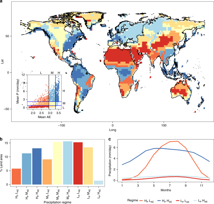
qualitatively, we plotted various characteristics of the resulting regimes in Fig. 1. The spatial distribution of regimes based on precipitation means and seasonal variations is shown in

Fig. 1a. The percentage of land occupied by each classified regime is shown in Fig. 1b. The plot region in the legend is divided into nine zones, each of which is delineated with two

intersecting dividing lines that pass through the limits of the respective thresholds of the two variables. Global land regions are classified into nine regimes based on percentiles

thresholds (i.e., <30th—Low; 30–70th—Moderate; >70th—High) of seasonal variation (as defined by AE) and annual mean precipitation during the 1971–2000 reference period (See “Methods”).

We chose four critical zones (HpHAE, LPHAE, LPLAE, HPLAE) to illustrate extreme scenarios based on combinations of either low (<Pr30) and high (>Pr70) variation and mean value of

precipitation. Here, HAE represents higher AE values, which implies lower seasonal variation. The spatially aggregate precipitation climatology of the selected four regimes is detailed in

Fig. 1c. For each grid, the month with lowest rainfall is plotted as starting month for rainfall. Regime HpHAE witnesses a higher precipitation rate and lower intra-annual variability (i.e.,

high AE). As a result, the precipitation is uniformly distributed, indicating perennial water supply for both human and ecological needs3,31. On the contrary, regime HPLAE presents a

scenario (high precipitation and high variability), where most of the precipitation is concentrated in a limited number of months. As a result, excess water needs to be stored to prevent

floods as well as to enhance water supply for stakeholders in dry months. In low-precipitation regimes (LPHAE and LPLAE), virtual water transfers and drought-tolerant crops are prevalent32.

However, regions with less precipitation and higher AE (LPHAE) are perennial in nature. Regions characterized by a combination of lower precipitation and AE (LPLAE) are arid in nature,

indicating water resources availability is extremely low. Therefore, based on these principles, the remaining regimes have precipitation conditions between these extreme limiting cases. The

spatial distribution of regimes across global land is found to be as follows: regime HPLAE and MPLAE can be found mostly in the Indian subcontinent, Northeast Asia, Northern Australia, and

much of north-central and south-central Africa, covering land area of ~15%. These regions are influenced mostly by monsoons33. Regime HPMAE and HPHAE mostly occupy eastern North America,

Northern South America, central Africa, Western Europe, and South Eastern Asia, occupying a combined land area of 24%. These regions are mostly moist forest areas. Regime MPMAE spans across

most of central North America and is scattered in western parts of South America and Northern and central Asia, Southern part of Africa and Southern Australia amounting to ~15% of land area.

Regime MPHAE occupies most of European Continent and further extends to western Russia occupying 16% of the total land area. Regime LPLAE occupies Northern Africa, the Middle East, and

further extends to central Asia. In addition, central Australia, the interior western United States and central western South America are classified as belonging to LPLAE, occupying a land

area of 15%. LPMAE is mostly confined to the Northern parts of North America and Siberia region occupying ~13% of land area. Finally, regime LPHAE is confined to a small region in the

central Russian region. TRENDS IN ANNUAL CHANGES OF PRECIPITATION AND EVAPORATION Precipitation and evaporation projections from Coupled Model Intercomparison Project Phase 5 (CMIP5) models

are aggregated over these nine precipitation regimes. We evaluate linear trends over the 21st century (2005–2100) using Bayesian model averaging (BMA) (31_–_32, see “Methods”) applied to

both annual means and seasonal variation in precipitation and evaporation for three future scenarios (representative concentration pathway (RCP) 2.6, 4.5, and 8.5). The changes in

BMA-weighted future annual precipitation and evaporation totals and seasonal variability for the RCP scenarios 2.6, 4.5, and 8.6 are shown in Fig. 2a, b, respectively (note that the

horizontal axis scales are different for both panels in Fig. 2a, b). In Fig. 2a, the change in annual precipitation total (TOTP) indicates an increase in precipitation in all regimes, with

the least increase in regime LPLAE, In addition, a proportional relationship was observed in terms of an increase in the precipitation magnitude with an increase in the emission forcing. In

addition, in precipitation regimes LPHAE, MPHAE, and HPHAE that are characterized by a relatively consistent water supply, the TOTP exhibit a higher magnitude of precipitation increase

compared with those regimes characterized by a moderate and high seasonal variability. Conversely, regions LPLAE, MPLAE, and HPLAE with inconsistent water supplies exhibit a lower magnitude

of precipitation increase. The highest magnitude increase is evident in regime HPHAE, which is characterized by high volumes of consistent water supply in which RCP 8.5 exhibits an increase

of 1.3 mm/year, followed by RCP 4.5 exhibiting 0.7 mm/year and RCP 2.6 exhibiting 0.25 mm/year. In addition, a larger uncertainty in the case of GCM model use is evident in precipitation

regime HPHAE. Similar to TOTP, an increase in the annual evaporation total (TOTE) is observed in all regimes with the lowest increase observed in regime LPLAE. In addition, a direct

proportional relationship is also evident here; the higher emission scenarios exhibit a higher magnitude of increased evaporation. As in the case of TOTP, TOTE in the precipitation regimes

of LPHAE, MPHAE, and HPHAE that are characterized by relatively consistent water supply exhibit a higher magnitude of evaporation increase. The greatest change is evident in regime MPHAE,

which is characterized by moderate precipitation but low seasonal variability. In this regime, RCP 8.5 exhibits an increase of 0.68 mm/year, followed by RCP 4.5 with an increase of 0.4 

mm/year and RCP 2.6 with an increase of 0.19 mm/year. We observe that the changes in magnitude of TOTE are generally less uncertain than those in precipitation. The decrease in AEP indicates

an increase in the seasonal variability of precipitation in the regimes LPLAE, MPLAE, and HPLAE for all RCP scenarios as detailed in Fig. 2b. Although a negligible trend in RCP 2.6 is

observed in case of regimes HPMAE, HPHAE, and MPMAE, a significant increase in variability was observed in the other scenarios for these three regimes. However, although a negligible

positive trend is observed in regimes LPMAE and LPHAE for RCP 2.6, the other scenarios exhibit a decrease in variability. Regime MPHAE, which is characterized by moderate and consistent

water supply exhibits a negligible change in all scenarios. Further, the changes in AEE are not as substantial as those in AEP. No significant trends are observed in AEE for regimes HPHAE,

HPMAE, HPLAE, and MPLAE. In addition, decrease in variability of evaporation is evident in regime LPHAE, LPMAE, MPHAE, and MPMAE. The higher emission scenarios display greater change in

magnitude for AEE. Unlike with precipitation variability, there is a pattern of decreased variability exhibited by AEE. These contrasting future projection changes in precipitation and

evaporation may result in spatially variable monthly WA (i.e., P–E)6,31,34. To further assess the robustness of our results, we also computed the grid-wise trends as shown in Supplementary

Figure 1 for RCP 8.5 scenario. Based on this spatially explicit analysis, we see that precipitation variability is increasing over a substantially greater region (~35.6% of the land surface)

than it is decreasing (~4% of the land surface). In addition, the spatial analysis indicates that this increase in variability in more prominent in regions with high variability.

Evaporation variability, conversely, is decreasing over a substantially greater region (~36% of the land surface) than it is increasing over (~6% of the land surface). Therefore, both these

analyses suggested an overall trend toward increasing precipitation variability along with decreasing evaporation variability, reinforcing our main conclusions. As these metrics aggregate

the monthly distributions of precipitation and evaporation at the annual scale obscuring seasonal behavior, it is worthwhile to additionally investigate, as described below, how these

changes are reflected in the monthly distribution of available water (determined as the difference between precipitation and evaporation—See “Methods”). PRECIPITATION AND EVAPORATION ROLE IN

AVAILABLE WATER CHANGE We determine which seasonal components have contributed to altering the monthly distribution of WA (precipitation–evaporation) for each of these scenarios (See

“Methods”). The BMA-weighted historical (1971–2000) monthly WA distribution and future projections (2070–2099) for each regime are shown in Fig. 3 for each of the scenarios. The projected

future monthly distribution of WA for the wet seasons (8th–10th month) demonstrates that the wet season becomes wetter, a pattern that is increasingly evident in regimes LPHAE, MPHAE, and

HPHAE with a consistent water supply albeit less evident in regimes LPLAE and MPLAE with an inconsistent water supply (regime HPLAE exhibits a minor increase in available water). So, while

seasonally variable regimes becoming more variable in terms of precipitation, that is not the case for WA, perhaps owing to competing effects between evaporation and precipitation. The low

precipitation of regime LPLAE exhibits the least noticeable change in monthly available water, unlike the high precipitation of regime HPLAE, wherein a more noticeable increase in available

water is evident during the wet season. This pattern is also sensitive to the change in radiative forcing, with greater radiative forcing corresponding to greater changes. Therefore, in

regions where water supply is constrained by low-precipitation amounts and a more uneven distribution (low AE), changes in precipitation and evaporation do not affect the available water as

they are more water-limited in nature. In regions with a more even distribution, however, there is a greater effect. Overall, these results indicate that the changes in monthly WA

distribution are dependent on both the particular regime and the radiative forcing. The corresponding changes in precipitation and evaporation (relative to the historical period) during the

wet and dry seasons for three future emission scenarios (RCP 2.6, 4.5, 8.5) are presented in Fig. 4, illustrating the competition between water and energy balance at the seasonal scale. The

role played by both wet and dry seasons in changing WA are examined in Fig. 4. In regions with high AE values (i.e., LPHAE, MPHAE, and HPHAE), higher increases in evaporation can be observed

in comparison with the moderate and low AE regions, especially in the RCP 8.5 scenario. These changes are significant in the wet season but not the dry season. As noted earlier, higher

emission scenarios show more pronounced evaporation increases. In the case of precipitation, regimes with high AE values in both dry and wet seasons display a pattern of increase similar to

that in evaporation. But these changes are again only statistically significant in the wet season. Although greater changes in precipitation are evident in the dry season, the greater spread

among models in that case hinders any confident conclusions. The increasing wet and dry season precipitation and evaporation provide an explanation for the changes in available water as

defined by the difference between precipitation and evaporation (precipitation–evaporation). In regimes where the relative magnitude of the increase in evaporation is less than that in

precipitation, a significant increase in WA is observed. Such is the case with high AE regions in wet season. This increase can thus be attributed to a larger increase in precipitation than

in evaporation. In addition, regions with higher AE exhibit a greater increase in WA, which imply the potential for increased flood risk in regions such as Western Europe35, North America36,

and South Eastern Asia that show less-seasonal variation16. In the case of the dry season, an increase in WA is found in RCP 8.5 scenarios for regimes LPMAE, MPMAE, and HPHAE but it is not

statistically significant. The results in these cases are inconclusive owing to the large spread among models. This finding further highlights the interdependent role of evaporation and

precipitation in changing seasonal WA. Previous studies based on spatially explicit analyses have shown that the dry seasons are becoming drier in some locations around the globe9. Our

spatial analysis in case of RCP 8.5 scenario also indicates a decrease in P–E in Europe and northern part of North America (Supplementary Fig. 2) in agreement with Kumar et al.10,37.

DISCUSSION Coupled changes in seasonal variation (as measured by AE) and annual mean precipitation and evaporation significantly impact the spatio-temporal distribution of WA. By using

appropriate thresholds applied to seasonal variations and annual means of historical precipitation data, nine land regions were identified that are characterized by different water supply

regimes. Spatially aggregated future trends over these regimes as applied to the CMIP5 future projections indicate an increase in precipitation annual means in all land regimes across the

globe, with higher increases in RCP 8.5 as reported in previous studies6,7,8,38. Most strikingly, annual mean evaporation is found to be increasing in all regimes, indicating a pattern of

intensified response to increased water demand across all regions. Furthermore, an increase in seasonal precipitation variation is observed, especially in regions that already exhibit

greater seasonal variation in precipitation. This indicates a pattern of seasonally variable regimes becoming more variable regarding precipitation. This pattern is consistent with

previously reported observations of the wet season becoming more wet and the dry season becoming more dry39,40. In the case of wet seasons becoming wet, vertical moisture advection and

evaporation play a key role40,41. Therefore, we anticipate that the observed pattern may be owing to regional changes in moisture advection and evaporation. However, we do not observe such a

pattern in the seasonal variability of evaporation. We found a decrease in seasonal evaporation variation in various regimes of the global land area. This would imply that regions that

already have inconsistent water supply owing to high seasonal variation in precipitation might experience even more inconsistent WA. Similar to what is observed with precipitation, an

increase in the annual mean evaporation (TOTE) is observed in all regimes with the smallest increase observed in regime LPLAE, as found in previous studies41. Increases in annual mean

evaporation over the land surface can be attributed to the increase in temperature in the CMIP5 future projections42 and also to increase in precipitation. The seasonal changes in

evaporation, however, are tied to corresponding seasonal changes in surface relative humidity contrast42,43. Also, the increase in TOTE is smaller than in TOTP, a finding that is consistent

with previous studies31,42. We also examined the projected monthly distribution of WA as measured by precipitation minus evaporation (P–E) across the classified nine precipitation regimes.

Our results highlight a clear signal of increased WA in the wet season especially in regimes of less-seasonal variation in precipitation. We assessed the role of precipitation and

evaporation characteristics in the changing monthly distributions of WA. Our results indicate that the increases in WA in wet seasons is controlled by changes in both precipitation and

evaporation. The combination of changes in precipitation and evaporation might result in an overall increase in WA, which is more pronounced during the wet season and is expected to yield

spatially variable annual WA consistent with previous studies37,44,45. However, we show that these changes may also be dependent upon the specific regime as determined by both seasonal

variation and mean precipitation changes. Even though our results indicate changes in long-term WA, it is unclear what implications our findings might hold for hydrologic extremes, owing to

limitations in the ability of current generation coupled climate models to capture the key drivers of persistent weather extremes46,47. Overall, these changes in precipitation

characteristics impact not only annual WA but also its spatio-temporal distribution. Concomitant changes in the mean and seasonal variation in precipitation may imply significant and varied

shifts in phenology48,49, reservoir management3, and ecosystem function depending upon the water supply regimes. The framework provided by our study complements traditional approaches used

to study seasonal variability in different hydroclimatic regimes50,51. Future efforts will use this framework to quantitatively assess the implications of projected changes in seasonal and

annual mean precipitation on streamflow regimes, providing further relevance to issues involving societal water use and demand. DATA Observed precipitation gridded data from GPCC52 at a

resolution of 2.5 × 2.5◦ for the period of 1901–2005 at monthly scale is used. Conversely, the observed terrestrial evaporation measurements were obtained from Global Land Evaporation

Amsterdam Model (GLEAM) data set available for the period of 1980–201553 at a daily scale. This data set incorporates the Priestley and Taylor equation to calculate the potential evaporation

based on observations of surface net radiation and near surface air temperature. A multiplicative evaporative stress factor estimated from satellite estimates is then used to convert the

calculated potential evaporation values to actual evaporation. A more-detailed calculation procedure is available in the work of Martens et al.53. The future projected data from 21 different

general climatic models under the CMIP5 version for three different RCP scenarios are used. Each of these scenarios are distinguished by their radiative forcing increases by the end of the

current century (RCP 2.6, 4.5, and 8.5) relative to pre-industrial values (Supplementary Table 1). These scenarios correspond roughly to a 2 °C stabilization, and 3.5 °C and 5 °C global

temperature increase, respectively, by the end of the century. These CMIP5 models are selected based on the common availability of both precipitation and evaporation variables for historical

and projected scenarios. METHODS ANNUAL PRECIPITATION AND EVAPORATION CHARACTERISTICS After acquisition of the data, both the observed and modeled data are interpolated to a common 2.5 × 

2.5° grid from their respective original grids. We assessed the seasonal variation of monthly precipitation and evaporation using an information theory metric called as AE. Unlike the

parametric coefficient of both variation and standard deviation, this metric is non-parametric and may even encompass high-order moments3. Moreover, information theory metrics have been

widely used as a measure of rainfall seasonality in both hydrologic and climatological contexts3,24,26,27. Therefore, to estimate AE for either precipitation or evaporation over a year _k_,

the aggregated annual quantities during the 12 months indexed are computed by summing the monthly values (_x_) over all the months in a year as $$X = \mathop {\sum}\limits_{i = 1}^{12}

{x_i}$$ (1) where _X_ is the aggregated value of either the precipitation or evaporation. Subsequently, the AE is calculated as $$AE = - \mathop {\sum}\limits_{i = 1}^{12} {\left( {x_i/X}

\right)\log _2\left( {x_i/X} \right)}$$ (2) By definition, both Eqs. (1) and (2) state that when either the amount of annual precipitation or evaporation is quite evenly apportioned to each

of the 12 months with the probability of 1/12, Eq. (2) assumes the maximum value of log212. Conversely, the minimum value of AE = 0 occurs when the apportionment is extended to only 1 month

of the 12 month cycle with a probability of 1, thus indicating the assumption of a new value by AE within a finite range of 0 and log212. Therefore, in a year, the less variable the monthly

precipitation or evaporation, the higher the AE value. Using this definition, the seasonal variability of precipitation (AEP) and evaporation (AEE) is estimated for the study period. The

aggregation of both the precipitation (TOTP) and evaporation (TOTE) is then used to calculate the annual precipitation and evaporation during these 12 months. DEFINITION OF GLOBAL

CLASSIFICATION OF PRECIPITATION REGIMES The existing atmospheric climate classifications are based on broad precipitation, temperature, evapotranspiration, and biosphere

characteristics21,22,23. However, even though the seasonal variability significantly changes across the global land regions26,27, it is often not considered for classification from a

non-parametric standpoint. For instance, the occurrence of substantial precipitation with an even monthly distribution will indicate a consistent and adequate supply of atmospheric water

throughout the year. Similarly, an occurrence of substantial precipitation with an uneven monthly distribution will indicate surplus water supply during a particular period of a given year

and deficit water supply during another period in a given year. Therefore, a failure to consider the seasonal variability of precipitation magnitude may well lead to a misrepresentation of

the actual water supply conditions. Therefore, in this study, in addition to the precipitation magnitude, the seasonal variability was also included for purposes of classifying the global

land regions into distinct water supply regimes. Here, the global land was divided into nine regimes of varying magnitudes of observed annual precipitation and seasonal variability based on

the period between the years 1971 and 2000. These regimes are derived based on a combination of seasonal variabilities (i.e., AE) and magnitude using the threshold concept: with high

(>Pr70), moderate (between Pr30 and Pr70) and low (<Pr30), in which Pri represents the ith percentile of either the annual magnitude or the seasonal variability. The use of the 30th

and 70th percentiles is based upon the wet and dry region definitions adopted by Allan et al.54 and subsequently implemented in Liu and Allan55. A similar threshold based classification of

various dry and wet global regions has been used elsewhere with success56,57,58. In using this approach, we have coupled the characteristics of both annual magnitude and seasonal variability

into distinct regimes based on global percentile thresholds. As a result, this definition can capture the precipitation characteristics that might have been previously omitted in those

definitions based on absolute thresholds, separate precipitation magnitude and seasonal variability considerations and regional definitions59. The classification of these regimes also do not

explicitly consider the natural landscape (e.g., rainforest, deserts) or the human-experienced climate events (e.g., monsoons) as suggested by Trewartha54. As we base our analysis on both

precipitation and evaporation, this scheme provides a necessary and rather simple configuration for the relative assessment of spatially aggregated changes in both precipitation and

evaporation characteristics for this study. All the derived precipitation and evaporation characteristics for CMIP5 as well as the observed data over these regimes are spatially aggregated.

BAYESIAN MODEL AVERAGING As the CMIP5 models exhibit varying levels of accuracy regarding simulating historical hydrologic cycles, the BMA methodology52 is utilized to assign higher weights

to better performing models. For this purpose, we computed the yearly precipitation and evaporation totals and AE, from the CMIP5 models and observed data sets, i.e., precipitation from GPCC

and evaporation dataset from GLEAM over each precipitation regime. Then the BMA approach is utilized to determine the optimal weights for each CMIP5 model on their ability to replicate the

spatial patterns of TOTP, TOTE, AEP, and AEE. The BMA approach calculates ensemble of the considered CMIP5 models by assigning weights based on the performance of models in comparison with

the observations52,60. In this approach, the probability density function (_g_) of our interest variable, \(Y \in \left\{ {P,E,AE_P,AE_E} \right\}\) from the observed data, which is

conditioned upon the 21 CMIP5 simulations is expressed as: $$g\left( {Y|Y_1,...,Y_{21}} \right) = \mathop {\sum}\limits_{i = 1}^{21} {w_if\left( {Y|Y_i} \right)}$$ (3) where _w__i_ is the

optimal weight for the _i_th CMIP5 model, _f_(_Y_|_Y__i_) is a PDF of the gamma distribution of _Y__i_. The general selection of the BMA mixture probability distribution is normal with the

gamma distributions based on the suggestion of Vrugt et al.60 and Raftery et al.52. Therefore, in this study, a separate analysis is undertaken for both of the prior distributions. The BMA

ensemble weighted mean and standard deviation is thus expressed as: $$En = \mathop {\sum}\limits_{i = 1}^{21} {w_i * Y_i}$$ (4) $$RMSD = \left[ {\mathop {\sum}\limits_{i = 1}^{21} {w_i\left(

{Y_i - EN} \right)} } \right]^{1/2}$$ (5) ESTIMATION OF BMA WEIGHTS The optimal weights w_i_, _i_ = 1, …, 21 are estimated with a maximum log-likelihood function, which is expressed as:

$$l\left( {w_1, \ldots ,w_{21}} \right) = \mathop {\sum}\limits_{j = 1}^N {\log \left( {\mathop {\sum}\limits_{i = 1}^{21} {w_ig\left( {Y_j\left| {Y_{i,j}} \right.} \right)} } \right)}$$ (6)

where _j_ = {1, … _N_} are observations of the considered variable. Regarding precipitation, we use the mean annual estimates from 1971 to 2000 for estimating the optimal weights. Regarding

evaporation, we only use the annual characteristics from 1980 to 2005. A Markov Chain Monte Carlo algorithm60, which maximizes the log-likelihood function is used for estimating the

weights. This algorithm in turn generates _N_ different Markov Chains, placed separately as rows with each chain represented as a 22-dimensional vector _θ_ = {_w__1__, w__2__,…, w__21__,

σ__2_}. The candidate maximum likelihood point is then sampled from a prescribed distribution, depending on the precipitation regime. Next, in accordance with the Metropolis acceptance

probability, the candidate maximum likelihood point is either accepted or rejected. If accepted, the chain moves to the next candidate model; otherwise the chain repeats the process until

the optimal weight for the candidate model is estimated. Clearly, the BMA weights obtained through maximum likelihood using this procedure is comparatively more accurate than the weights

obtained using the Expectation–Maximization (EM) algorithm recommended by Raftery et al.52. A thorough description of this algorithm is presented in Vrugt et al.60. The estimated BMA weights

are listed in Supplementary Table 2. PERFORMANCE AND EVALUATION OF BMA MULTIMODEL ENSEMBLES OVER PRECIPITATION REGIMES The performance of the BMA multimodel ensemble was assessed in terms

in replicating the spatial pattern across the land regions. After obtaining the optimal weights (shown in Supplementary Table 2), we computed the multimodel ensemble using Eq. (4) and

evaluated the performance by the metrics of the Pearson correlation. The results indicate that in terms of the TOTP, TOTE, an _R_2 values of 0.94 and 0.92, respectively, is obtained. Whereas

in case of AEP and AEE an _R_2 of 0.91 and 0.85 are obtained. These values further indicate that ensemble mean of the 21 GCMs, which are studied could adequately replicate the spatial

patterns. ASSESSMENT OF PROJECTED CHANGES The projected changes of TOTP, TOTE, AEP, and AEE were determined using the non-parametric Theil-Sen estimator61. We first estimated the linear

trends using Theil-Sen estimator (\(\Delta Y\)) and the BMA ensemble trend with an uncertainty is expressed as $$\Delta Y_{BMA} = \mathop {\sum}\limits_{i = 1}^{21} {w_i * \Delta Y_i}$$ (7)

$$\Delta Y_{RMSD} = \left[ {\mathop {\sum}\limits_{i = 1}^{21} {w_i\left( {\Delta Y_i - \Delta Y_{BMA}} \right)} } \right]^{1/2}$$ (8) thus, permitting the estimates of the upper and lower

confidence limits as: $$\Delta Y_{UC} = \Delta Y_{BMA} + 2 * \Delta Y_{RMSD}$$ (9) $$\Delta Y_{LC} = \Delta Y_{BMA} - 2 * \Delta Y_{RMSD}$$ (10) If the changes are distributed as a Gaussian

density function, then these bounds imply a ~95% confidence interval. AVAILABLE WATER The difference between monthly precipitation and evaporation variables is deemed reliable for

approximating the potential available water for human and ecological consumption. Here, we estimate the average net available water in 1 month for the historical period of 1971–2000 and for

the future scenario of 2070–2099, which is expressed as: $$WA_{hist}^m = \frac{{\mathop {\sum}\nolimits_{y = 1970}^{2000} {\left( {r_{m,y} - e_{m,y}} \right)} }}{{30}}$$ (11) $$WA_{rcp}^m =

\frac{{\mathop {\sum}\nolimits_{y = 2070}^{2100} {\left( {r_{m,y} - e_{m,y}} \right)} }}{{30}}$$ (12) where _r__m,y_ and _e__m,y_ represent the precipitation and evaporation in month _m_ and

year _y_. We then compare the monthly net available water of historical and future scenarios (RCP 2.6, 4.5, and 8.5) from each GCM model through a spatial averaging over respective regimes.

The denominator 30 represents the total number of years taken into consideration. In case of WA, we used the averaged BMA weights for each model and estimated the monthly distribution of

WA. To explore the role of seasonal components in terms of altering the monthly climatology of available water seasonal variability within a hydrologic year, we first extracted wet and dry

precipitation and evaporation components. We assumed a 3-month period in which the maximum (minimum) of available water occurs as wet (dry) seasons40 using the same base period of 1971–2000.

We estimated the changes in both the wet and dry seasons as the difference between the future scenarios (2070–2099) and the mean historical (1971–2000) spatially aggregation over each

regime. The BMA weights were applied and the uncertainty was calculated using Eqs. (7–10). DATA AVAILABILITY The data sets analyzed during the current study are available at Earth System

Grid Federation (ESGF) Peer-to-Peer (P2P) enterprise system [https://esgf-node.llnl.gov/projects/esgf-llnl/]. The Observed monthly GPCC precipitation is available at

https://opendata.dwd.de/climate_environment/GPCC/html/fulldata-monthly_v2018_doi_download.html. The evaporation data set is available at https://www.gleam.eu/. CODE AVAILABILITY The

accompanying MATLAB source code for Bayesian model averaging utilized in this study is available at (http://faculty.sites.uci.edu/jasper/software). REFERENCES * Milly, P., Dunne, K. &

Vecchia, A. Global pattern of trends in streamflow and water availability in a changing climate. _Nature_ 438, 347–350 (2005). Article  ADS  CAS  Google Scholar  * Oki, T. and Kanae, S.

Global hydrological cycles and world water resources. _Science_ 313, 1068–1072 (2006). * Mishra, A. K., Özger, M. & Singh, V. P. Association between uncertainties in meteorological

variables and water-resources planning for the state of Texas. _J. Hydrologic Eng._ 16, 984–999 (2010). Article  Google Scholar  * Haddeland, I., et al. Global water resources affected by

human interventions and climate change. _Proc. Natl Acad. Sci._ https://doi.org/10.1073/pnas.1222475110 (2014). * Schewe, J., et al. Multimodel assessment of water scarcity under climate

change. _Proc. Natl Acad. Sci._ https://doi.org/10.1073/pnas.1222460110 (2014). * Knutti, R., & Sedláček, J. Robustness and uncertainties in the new CMIP5 climate model projections.

_Nat. Clim. Change_ https://doi.org/10.1038/nclimate1716 (2013). * Chadwick, R., Boutle, I., & Martin, G. Spatial patterns of precipitation change in CMIP5: why the rich do not get

richer in the tropics. _J. Clim._ https://doi.org/10.1175/JCLI-D-12-00543.1 (2013). * Polade, S. D., Pierce, D. W., Cayan, D. R., Gershunov, A., & Dettinger, M. D. The key role of dry

days in changing regional climate and precipitation regimes. _Sci. Rep._ https://doi.org/10.1038/srep04364 (2014). * Kumar, S., Lawrence, D. M., Dirmeyer, P. A., & Sheffield, J. Less

reliable water availability in the 21st century climate projections. _Earth’s Future_. https://doi.org/10.1002/2013EF000159 (2014). * Kharin, V. V., Zwiers, F. W., Zhang, X., & Wehner,

M. Changes in temperature and precipitation extremes in the CMIP5 ensemble. _Clim. Change_. https://doi.org/10.1007/s10584-013-0705-8 (2013). * Sillmann, J., Kharin, V. V., Zwiers, F. W.,

Zhang, X., & Bronaugh, D. Climate extremes indices in the CMIP5 multimodel ensemble: part 2. Future climate projections. _J. Geophys. Res._ https://doi.org/10.1002/jgrd.50188 (2013). *

Liu, W., & Sun, F. Projecting and attributing future changes of evaporative demand over China in CMIP5 climate models. _J. Hydrometeorol._ https://doi.org/10.1175/JHM-D-16-0204.1 (2017).

* Mueller, B., & Seneviratne, S. I. Systematic land climate and evapotranspiration biases in CMIP5 simulations. _Geophys. Res. Lett._ https://doi.org/10.1002/2013GL058055 (2014). *

Milly, P. C. & Dunne, K. A. Potential evapotranspiration and continental drying. _Nat. Clim. Change_ 6, 946 (2016). Article  ADS  Google Scholar  * Kundzewicz, Z. W., & Gerten, D.

Grand challenges related to the assessment of climate change impacts on freshwater resources. _J. Hydrol. Eng._ https://doi.org/10.1061/(ASCE)HE.1943-5584.0001012 (2014). * Arnell, N. W.,

& Gosling, S. N. The impacts of climate change on river flood risk at the global scale. _Clim. Change_. https://doi.org/10.1007/s10584-014-1084-5 (2016). * Gornall, J., et al.

Implications of climate change for agricultural productivity in the early twenty-first century. _Philos. Trans. R. Soci. London B: Biol. Sci_. https://doi.org/10.1098/rstb.2010.0158 (2010).

* Challinor, A. J., et al. A meta-analysis of crop yield under climate change and adaptation. _Nat. Clim. Change_. https://doi.org/10.1038/nclimate2153 (2014). * Keersmaecker, W., et al. How

to measure ecosystem stability? An evaluation of the reliability of stability metrics based on remote sensing time series across the major global ecosystems. _Glob. Change Biol._

https://doi.org/10.1111/gcb.12495 (2014). * Seddon, A. W., Macias-Fauria, M., Long, P. R., Benz, D., & Willis, K. J. Sensitivity of global terrestrial ecosystems to climate variability.

_Nature_. https://doi.org/10.1038/nature16986 (2016). * Kottek, M., Grieser, J., Beck, C., Rudolf, B., & Rubel, F. World map of the Köppen-Geiger climate classification updated.

_Meteorologische Zeitschrift_. https://doi.org/10.1127/0941-2948/2006/0130 (2006). * Holdridge, L. R. Determination of world plant formations from simple climatic data. _Science_.

https://doi.org/10.1126/science.105.2727.367 (1947). * Thornthwaite, C. W. “An approach toward a rational classification of climate.” _Geogr. Rev._ 38, 55–94 (1948). Article  Google Scholar

  * Feng, X., Porporato, A., & Rodriguez-Iturbe, I. Changes in rainfall seasonality in the tropics. _Nat. Clim. Change_. https://doi.org/10.1038/nclimate1907 (2013). * Rajah, K., et al.

Changes to the temporal distribution of daily precipitation. _Geophys. Res. Lett._ https://doi.org/10.1002/2014GL062156 (2014). * Pascale, S., Lucarini, V., Feng, X., Porporato, A., & ul

Hasson, S. Analysis of rainfall seasonality from observations and climate models. _Clim. Dyn._ https://doi.org/10.1007/s00382-014-2278-2 (2015). * Pascale, S., Lucarini, V., Feng, X.,

Porporato, A., & ul Hasson, S. Projected changes of rainfall seasonality and dry spells in a high greenhouse gas emissions scenario. _Clim. Dyn._

https://doi.org/10.1007/s00382-015-2648-4 (2016). * Miralles, D. G., et al. Global land-surface evaporation estimated from satellite-based observations. _Hydrol. Earth Syst. Sci._

https://doi.org/10.5194/hess-15-453-2011 (2011). * Zeng, Z., et al. A worldwide analysis of spatiotemporal changes in water balance‐based evapotranspiration from 1982 to 2009. _J. Geophys.

Res._ https://doi.org/10.1002/2013JD020941 (2014). * Becker, A., et al. A description of the global land-surface precipitation data products of the Global Precipitation Climatology Centre

with sample applications including centennial (trend) analysis from 1901-present. _Earth Syst. Sci. Data_. https://doi.org/10.5194/essd-5-71-2013 (2013). * Levang, S. J., & Schmitt, R.

W. Centennial changes of the global water cycle in CMIP5 models. _J. Clim._ https://doi.org/10.1175/JCLI-D-15-0143.1 (2015). * Loveland, T. R. et al. Development of a global land cover

characteristics database and IGBP DISCover from 1 km AVHRR data. _Int. J. Remote Sens._ 21, 1303–1330 (2000). Article  Google Scholar  * Wang, B., & Ding, Q. Changes in global monsoon

precipitation over the past 56 years. _Geophys. Res. Lett._ https://doi.org/10.1029/2005GL025347 (2006). * Greve, P., et al. Global assessment of trends in wetting and drying over land.

_Nat. Geosci._ https://doi.org/10.1038/ngeo2247 (2014), * Alfieri, L., Burek, P., Feyen, L., & Forzieri, G. Global warming increases the frequency of river floods in Europe. _Hydrol.

Earth Syst. Sci._ https://doi.org/10.5194/hess-19-2247-2015 (2015). * Swain, S., & Hayhoe, K. CMIP5 projected changes in spring and summer drought and wet conditions over North America.

_Clim. Dyn._ https://doi.org/10.1007/s00382-014-2255-9 (2015). * Kumar, S., Allan, R. P., Zwiers, F., Lawrence, D. M., & Dirmeyer, P. A. Revisiting trends in wetness and dryness in the

presence of internal climate variability and water limitations over land. _Geophys. Res. Lett._ https://doi.org/10.1002/2015GL066858 (2015). * Lau, W. K. M., Wu, H. T., & Kim, K. M. A

canonical response of precipitation characteristics to global warming from CMIP5 models. _Geophys. Res. Lett._ https://doi.org/10.1002/grl.50420 (2013). * Chou, C., et al. Increase in the

range between wet and dry season precipitation. _Nat. Geosci._ https://doi.org/10.1038/ngeo1744 (2013). * Chou, C., & Lan, C. W. Changes in the annual range of precipitation under global

warming. _J. Clim._ https://doi.org/10.1175/JCLI-D-11-00097.1 (2012). * Laîné, A., Nakamura, H., Nishii, K., & Miyasaka, T. A diagnostic study of future evaporation changes projected in

CMIP5 climate models. _Clim. Dyn._ https://doi.org/10.1007/s00382-014-2087-7 (2014). * Greve, P. and Seneviratne, S. Assessment of future changes in water availability and aridity.

_Geophys. Res. Lett._ https://doi.org/10.1002/2015GL064127 (2015). * Richter, I., & Xie, S. P. Muted precipitation increase in global warming simulations: a surface evaporation

perspective. _J. Geophys. Res._ https://doi.org/10.1029/2008JD010561 (2008). * Liepert, B. G., Previdi, M. Inter-model variability and biases of the global water cycle in CMIP3 coupled

climate models. _Environ. Res. Lett._ https://doi.org/10.1088/1748-9326/7/1/014006 (2012). * Roderick, M., Sun, L. F., Lim, W. H., and Farquhar, G. D. A general framework for understanding

the response of the water cycle to global warming over land and ocean. _Hydrol. Earth Syst. Sci._ https://doi.org/10.5194/hess-18-1575-2014 (2014). * Mann, M. E., et al. Influence of

anthropogenic climate change on planetary wave resonance and extreme weather events. _Sci. Rep._ https://doi.org/10.1038/srep45242 (2017). * Mann, M. E., et al. Projected changes in

persistent extreme summer weather events: the role of quasi-resonant amplification. _Sci. Adv_. https://doi.org/10.1126/sciadv.aat3272 (2018). * Huxman, T. E. et al. Precipitation pulses and

carbon fluxes in semiarid and arid ecosystems. _Oecologia_. https://doi.org/10.1007/s00442-004-1682-4 (2004). * Cleland, E. E., Chuine, I., Menzel, A., Mooney, H. A. & Schwartz, M. D.

Shifting plant phenology in response to global change. _Trends Ecol. Evol_. https://doi.org/10.1016/j.tree.2007.04.003 (2007). * Maruyama, T., Kawachi, T. & Singh, V. P. Entropy-based

assessment and clustering of potential water resources availability. _J. Hydrol._ 309, 104–113 (2005). Article  ADS  Google Scholar  * Kawachi, T., Maruyama, T. & Singh, V. P. Rainfall

entropy for delineation of water resources zones in Japan. _J. Hydrol._ 246, 36–44 (2001). Article  ADS  Google Scholar  * Raftery, A. E., Gneiting, T., Balabdaoui, F. & Polakowski, M.

Using Bayesian model averaging to calibrate forecast ensembles. _Monthly weather Rev._ 133, 1155–1174 (2005). Article  ADS  Google Scholar  * Martens, B., et al. GLEAM v3: satellite-based

land evaporation and root-zone soil moisture. _Geosci. Model Dev._ https://doi.org/10.5194/gmd-10-1903-2017 (2017). * Trewartha, G. T. _An introduction to weather and climate_. (Mcgraw-Hill

Book Company, Inc, New York; London, 1943). Google Scholar  * Liu, C., & Allan, R. P. (2013). Observed and simulated precipitation responses in wet and dry regions 1850–2100. _Environ.

Res. Lett._ https://doi.org/10.1088/1748-9326/5/2/025205, (2013). * Allan, R. P., Soden, B. J., John, V. O., Ingram, W., & Good, P. Current changes in tropical precipitation. _Environ.

Res. Lett._ https://doi.org/10.1088/1748-9326/5/2/025205 (2010). * Polson, D., Hegerl, G. C., Allan, R. P., & Sarojini, B. B. Have greenhouse gases intensified the contrast between wet

and dry regions?. _Geophys. Res. Lett._ https://doi.org/10.1002/grl.50923 (2013). * Donat, M. G., Lowry, A. L., Alexander, L. V., O’Gorman, P. A., & Maher, N. More extreme precipitation

in the world’s dry and wet regions. _Nat. Clim. Change_ https://doi.org/10.1038/nclimate2941 (2016). * De Castro, M., Gallardo, C., Jylha, K., & Tuomenvirta, H. The use of a climate-type

classification for assessing climate change effects in Europe from an ensemble of nine regional climate models. _Clim. Change_. https://doi.org/10.1007/s10584-006-9224-1 (2007). * Vrugt, J.

A. Markov chain Monte Carlo simulation using the DREAM software package: theory, concepts, and MATLAB implementation. _Environ. Model. Softw._ https://doi.org/10.1016/j.envsoft.2015.08.013

(2016). * Wilcox, R. R. Introduction to robust estimation and hypothesis testing. (Academic press, Amsterdam, 2011). MATH  Google Scholar  Download references ACKNOWLEDGEMENTS This study was

supported by the National Science Foundation (NSF) award # 1653841. AUTHOR INFORMATION AUTHORS AND AFFILIATIONS * Glenn Department of Civil Engineering, Lowry Hall, Clemson University,

Clemson, SC, 29634-0911, USA Goutam Konapala & Ashok K. Mishra * Environmental Sciences Division, Oak Ridge National Laboratory, Oak Ridge, TN, 37831, USA Goutam Konapala * Climate

Change Science Institute, Oak Ridge National Laboratory, Oak Ridge, TN, 37831, USA Goutam Konapala * Water program, International Institute for Applied Systems Analysis, Schlossplatz 1,

A-2361, Laxenburg, Austria Yoshihide Wada * Department of Meteorology and Atmospheric Science, 502 Walker Building, Pennsylvania State University, University Park, PA, 16802, USA Michael E.

Mann Authors * Goutam Konapala View author publications You can also search for this author inPubMed Google Scholar * Ashok K. Mishra View author publications You can also search for this

author inPubMed Google Scholar * Yoshihide Wada View author publications You can also search for this author inPubMed Google Scholar * Michael E. Mann View author publications You can also

search for this author inPubMed Google Scholar CONTRIBUTIONS A.M conceived the idea, and G.K. performed all analyses. Y.W. and M.M. contributed to the discussion and writing of the results

along with G.K. and A.M. CORRESPONDING AUTHOR Correspondence to Ashok K. Mishra. ETHICS DECLARATIONS COMPETING INTERESTS The authors declare no competing interests. ADDITIONAL INFORMATION

PEER REVIEW INFORMATION _Nature Communications_ thanks the anonymous reviewer(s) for their contribution to the peer review of this work. PUBLISHER’S NOTE Springer Nature remains neutral with

regard to jurisdictional claims in published maps and institutional affiliations. SUPPLEMENTARY INFORMATION SUPPLEMENTARY INFORMATION RIGHTS AND PERMISSIONS OPEN ACCESS This article is

licensed under a Creative Commons Attribution 4.0 International License, which permits use, sharing, adaptation, distribution and reproduction in any medium or format, as long as you give

appropriate credit to the original author(s) and the source, provide a link to the Creative Commons license, and indicate if changes were made. The images or other third party material in

this article are included in the article’s Creative Commons license, unless indicated otherwise in a credit line to the material. If material is not included in the article’s Creative

Commons license and your intended use is not permitted by statutory regulation or exceeds the permitted use, you will need to obtain permission directly from the copyright holder. To view a

copy of this license, visit http://creativecommons.org/licenses/by/4.0/. Reprints and permissions ABOUT THIS ARTICLE CITE THIS ARTICLE Konapala, G., Mishra, A.K., Wada, Y. _et al._ Climate

change will affect global water availability through compounding changes in seasonal precipitation and evaporation. _Nat Commun_ 11, 3044 (2020). https://doi.org/10.1038/s41467-020-16757-w

Download citation * Received: 10 October 2018 * Accepted: 19 May 2020 * Published: 23 June 2020 * DOI: https://doi.org/10.1038/s41467-020-16757-w SHARE THIS ARTICLE Anyone you share the

following link with will be able to read this content: Get shareable link Sorry, a shareable link is not currently available for this article. Copy to clipboard Provided by the Springer

Nature SharedIt content-sharing initiative