Temporal aiming | Light: Science & Applications

ABSTRACT Deflecting and changing the direction of propagation of electromagnetic waves are needed in multiple applications, such as in lens–antenna systems, point-to-point communications and

radars. In this realm, metamaterials have been demonstrated to be great candidates for controlling wave propagation and wave–matter interactions by offering manipulation of their

electromagnetic properties at will. They have been studied mainly in the frequency domain, but their temporal manipulation has become a topic of great interest during the past few years in

the design of spatiotemporally modulated artificial media. In this work, we propose an idea for changing the direction of the energy propagation of electromagnetic waves by using

time-dependent metamaterials, the permittivity of which is rapidly changed from isotropic to anisotropic values, an approach that we call _temporal aiming_. In so doing, here, we show how

the direction of the Poynting vector becomes different from that of the wavenumber. Several scenarios are analytically and numerically evaluated, such as plane waves under oblique incidence

and Gaussian beams, demonstrating how proper engineering of the isotropic—anisotropic temporal function of εr(t) can lead to a redirection of waves to different spatial locations in real

time. SIMILAR CONTENT BEING VIEWED BY OTHERS FOCUSING LIGHT INTO SCATTERING MEDIA WITH ULTRASOUND-INDUCED FIELD PERTURBATION Article Open access 02 August 2021 TIME REVERSED OPTICAL WAVES BY

ARBITRARY VECTOR SPATIOTEMPORAL FIELD GENERATION Article Open access 16 November 2020 SHAPING LIGHT IN 3D SPACE BY COUNTER-PROPAGATION Article Open access 09 September 2021 INTRODUCTION

Achieving arbitrary control of electromagnetic wave propagation has been of great interest within the scientific community for many years. It is well known that carefully engineered

spatially varying geometries and materials can be implemented to manipulate wave–matter interactions1. This spatial control of waves is, in fact, the mechanism behind the development of many

applications we often use on a regular basis, such as lenses, sensors and radars. The field of antennas has also benefited from this spatial control of wave propagation, where, for

instance, in its basic configuration, it is possible to change the direction of a transmitted wave by mechanically modifying the spatial location of the transmitter, a technique known as

_mechanical beam steering_2. To further improve the spatial control of waves and to manipulate wave–matter interactions at will, metamaterials (and metasurfaces as their two-dimensional (2D)

version) have been proposed in recent decades3,4. They have been demonstrated to provide engineering of their electromagnetic parameters, such as the permittivity (_ε_) and permeability

(_µ_), achieving extreme parameter values that are, e.g., negative5,6,7,8 or near-zero9,10,11,12,13,14. They have been studied and demonstrated in different wave mechanisms and spectral

bands ranging from acoustics, microwave and millimetre waves, terahertz waves and optics15,16,17,18,19. The freedom offered by metamaterials and metasurfaces, along with their compact

designs, has opened up new avenues to improve the performance of devices and to develop new technologies, such as mathematical operators20, antennas and lenses21,22,23,24, sensors25,26,27

and polarisation converters28,29,30. The _beam steering_ of electromagnetic waves has also benefited from the introduction of metamaterials, where it has been shown that electromagnetic

radiated beams can be redirected by changing the position of the source in a metalens–antenna system, by locally designing the phase of the unit cells in the metamaterials, or by real-time

tuning of the effective electromagnetic parameters of the metastructures31,32,33,34,35,36, among other techniques. These steering properties are important in different areas, such as in

point-to-point communications and radars, where the spatial aiming of targets is required. Metamaterials and metasurfaces have so far been studied mostly in the time-harmonic scenario, where

wave propagation is controlled by engineering geometries and materials in the spatial region, i.e., spatial inhomogeneity, in which the wave is travelling. Recently, the temporal modulation

of metamaterials has also gained growing attention within the scientific community37,38,39,40,41,42,43,44, as changing the electromagnetic properties (_ε_, _µ_) of metamaterials both in

space (_x, y, z_) and time (_t_) can offer full four-dimensional spatiotemporal control of wave–matter interactions. It is important to highlight that the interaction of electromagnetic

waves in a time-modulated medium has been of great interest in the scientific community for several decades, where, for instance, in the last century, it was considered a time-dependent

relative permittivity _ε__r_(_t_) that is rapidly changed in time from one positive value _ε__r_1 (greater than unity) to a different greater-than-unity positive value _ε__r_240,41. With

this configuration, it was demonstrated that a set of two waves is created at this temporal boundary, one of which is travelling forward (FW), and the other, backward (BW). Remarkably, an

analogy between this temporal and the spatial interface between two materials with different electromagnetic parameters was demonstrated, showing that the two waves created at a temporal

boundary (FW and BW) are the temporal equivalent/analogy to the transmitted and reflected waves in spatial interfaces. In this realm, temporal and spatiotemporal metamaterials have recently

been proposed and applied in several exciting and intriguing applications, such as effective medium theory45, inverse prisms46, nonreciprocity47,48, anti-reflection temporal coatings49,

frequency conversion50 and time reversal51. Motivated by the exciting possibilities and opportunities opened up by the spatiotemporal modulation of metamaterials in four dimensions (_x, y,

z, t_) and the importance of the beam steering of electromagnetic waves for different applications, in this work, we introduce the concept of temporal aiming as the temporal analogue of

spatial aiming. First, the fundamental physics of the proposed technique are presented, considering an oblique incident _p-_polarised monochromatic plane wave propagating in an unbounded

medium with a time-dependent permittivity _ε__r_(_t_). A temporal interface is introduced by changing the relative permittivity _ε__r_(_t_) from an isotropic positive value _ε__r_1 to an

anisotropic permittivity \(\overline{\overline {\varepsilon _{r2}}}\) = {_ε__r_2_x_, _ε__r_2_z_} (all with positive values greater than unity) at time _t_ = _t_1. In so doing, the wavenumber

_K_ is preserved before and after the temporal change, but the direction of the energy (Poynting vector _S_) is modified to a different angle compared with _K_. The dependence of the new

direction of the Poynting vector on the incident angle before the temporal change of _ε_ and the values of the permittivity tensor \(\overline{\overline {\varepsilon _{r2}}}\) is presented

and discussed. Next, we study more complex scenarios by using Gaussian beams under normal and oblique incidence to consider the case of multiple plane waves travelling in different

directions. With this set-up, it is demonstrated how the direction of the energy is modified to multiple angles when using an isotropic-to-anisotropic temporal boundary. Finally, the

temporal aiming technique is numerically demonstrated by using a narrowband wavepacket under oblique incidence. As will be shown, this transmitted wavepacket can be “ushered” and

“re-directed” in real time to reach different receivers placed at different spatial locations by properly engineering the _ε__r_(_t_) of the background medium. All the results presented here

are compared with numerical simulations, demonstrating good agreement with the design and analytical calculations. RESULTS TEMPORAL AIMING: ISOTROPIC-TO-ANISOTROPIC CHANGE IN _Ε__R_ First,

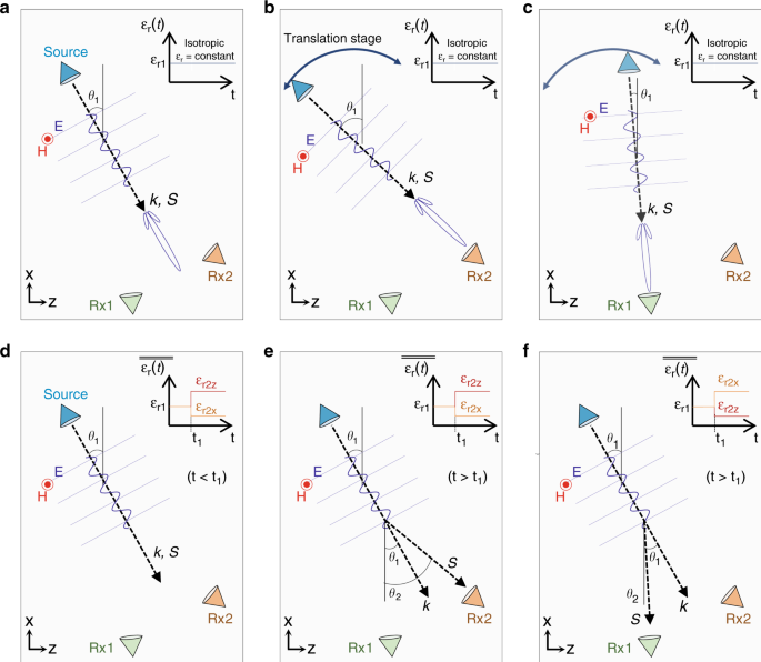
let us discuss the spatial scenario schematically described in Fig. 1a. In this case, we can consider a monochromatic continuous wave (CW) that is being emitted by a source located on the

_xz_ plane and tilted to an angle _θ__1_. The background medium is homogeneous, isotropic and time-independent, with a relative permeability _µ__r_(_t_) = _µ__r_1 and relative permittivity

_ε__r_(_t_) = _ε_r1 (see the inset of Fig. 1a). As is well known, the wave emitted from this source will also be tilted with the wavenumber _K_ and Poynting vector _S_ parallel, travelling

along the same direction defined by _θ_1. Now, let us place two receivers at two different spatial locations (Rx1 and Rx2), as schematically shown in Fig. 1a. As observed, this is not the

best scenario if one needs to send the emitted wave to either of the two receivers since the source is not aligned to Rx1 or to Rx2. However, as described in the introduction, the most

simple yet effective way to reach either Rx1 or Rx2 is to perform mechanical beam steering2,32. In this technique, the source is placed on a translation stage, and then spatially shifted to

different locations on the _xz_ plane to tilt the emitted wave to the correct angle _θ__1_ such that it reaches either Rx2 (Fig. 1b) or Rx1 (Fig. 1c). In addition to this technique, there

are other effective and more sophisticated alternatives that can be used to steer electromagnetic waves, such as phased arrays (in which the phase shifts between the antenna elements can be

changed in real time) and metamaterial-based antennas with tuneable properties31,34,36. In this context, steering electromagnetic waves is considered a key feature in applications where the

spatial aiming of targets is needed, such as radars and point-to-point communications, as explained before. The _spatial aiming_ described in Fig. 1a–c has been discussed considering the

time-harmonic scenario (frequency domain), taking into account that the relative permittivity and permeability of the background medium are constant [_ε__r_(_t_) = _ε__r_1, _µ__r_(_t_) = 

_µ__r_1]. With this in mind, one may ask the following: would it be possible to change the direction of the energy propagation of an emitted monochromatic CW plane wave in time by

considering a time-dependent permittivity _ε__r_(_t_) ≠ _ε__r_1 of the background medium? If such temporal aiming is possible, what type of function for _ε__r_(_t_) may we use to achieve it?

To answer these questions, in this work, we focus our attention on the rapid change in relative permittivity (approximately modelled mathematically as a “step function”), which is rapidly

modified in time from an initial value (equal to or greater than unity) εr1 to another greater-than-unity _ε__r_2 at a time _t_ = _t_1, considering that the fall/rise time is smaller than

the period T of the incident wave. (Strictly speaking, one needs to take into account the material dispersion in these scenarios. However, if we assume that the material resonance

frequencies are much larger than the frequency of operation, we can approximately assume the materials to be dispersionless). Let us study the case schematically shown in Fig. 1d. We again

assume a _p-_polarised monochromatic CW plane wave travelling in an unbounded medium with an incident angle _θ__1_. Let us first consider that the permittivity is time-dependent _ε__r_(_t_)

and is isotopically changed from a positive value _ε__r_1 to another positive value _ε__r_2. This scenario was studied in the last century, and it was shown that this _ε__r_(_t_) can induce

a temporal boundary/interface that generates a FW (temporal transmission) and a BW (temporal reflection) wave travelling with the same angle as that of the incoming wave, i.e., the

wavenumber _K_ is preserved while the frequency is changed from _f_1 to _f_2 = (\(\sqrt {\varepsilon _{r1}}\)/\(\sqrt {\varepsilon _{r2}}\))_f_1. This type of time-dependent _ε__r_(_t_) was

then recently used to propose exciting applications, such as time reversal and anti-reflection temporal coatings, as explained in the introduction. Nevertheless, since _K_ is the same before

(_t_ = _t_1−) and after (_t_ = _t_1+) the change in _ε_ from _ε__r_1 to _ε__r_2 and the direction of propagation for both _K_ and energy _S_ is not modified, it is straightforward to

conclude that this type of _ε__r_(_t_) is not suitable for the temporal aiming described in Fig. 1, since our aim is to redirect the energy of emitted waves to different receivers placed at

different spatial locations. Now, what if we change the relative permittivity εr from an isotropic value _ε__r_1 to an anisotropic permittivity tensor at _t_ = _t_1 such that

\(\overline{\overline {\varepsilon _{r2}}}\) = [_ε__r_2_x__, ε__r_2_z_] with _ε__r_2_x_ ≠ _ε__r_2_z_, both of which are positive, real-valued and greater-than-unity parameters? The schematic

representation of this _ε_(_t_) is shown in the inset of Fig. 1d. Note that here, we consider only the _z_ and _x_ components of the permittivity tensor since we have a TM polarisation with

the electric field lying on the _xz_ plane. Akbarzadeh et al. recently explored this function of _ε__r_(_t_) to create what they aptly called the “inverse prisms”, demonstrating that vector

_K_ is again preserved as the isotropic case while the frequency is modified, but this time with a value depending on the tensor \(\overline{\overline {\varepsilon _{r2}}}\) and the

incident angle _θ__1_46, hence their coined name, i.e., “inverse prism”. However, one may ask an intriguing question: what will happen to the Poynting vector _S_ in this scenario? Would it

be possible to exploit this isotropic-to-anisotropic temporal variation of ε(t) for temporal aiming, as we propose here? To answer these questions, let us analytically evaluate this case, as

shown in Fig. 1d. For _t_ < _t_1, the background medium is isotropic and homogeneous with relative permittivity and relative permeability values εr1 and µr1, respectively. With this

set-up (assuming the _e_(_iωt_) time convention), the magnetic and electric fields are \(H_1 = \hat ye^{i\left( {\omega _1t - k_xx - k_zz} \right)}\) and \(E_1 = \frac{1}{{\varepsilon

_{0}{\omega_1}\varepsilon _{r1}}}e^{i\left( {\omega _1t - k_xx - k_zz} \right)}\left[ {\begin{array}{*{20}{c}} {k_z} & 0 & { - k_x} \end{array}} \right]\), respectively, with ω1 = 

2π_f__1_, _k__x_ = –_k_cos_(θ__1__), k__z_ = _k_sin_(θ__1__)_, \(k = \omega _1/v_1\), \(v_1 = c/\sqrt {\mu _{r1}\varepsilon _{r1}}\) and _c_ being the velocity of light in vacuum. At _t_ = 

_t_1, the relative permittivity is changed to \(\overline{\overline {\varepsilon _{r2}}}\) = [_ε__r_2_x_, _ε__r_2_z_], and for completeness, the permeability is changed to _µ__r_2_y_. As

mentioned before, this temporal boundary creates a set of FW (E2+, H2+) and BW (E2−, H2−) waves, with the total electric and magnetic fields defined as E2 = E2+ + E2− and H2 = H2+– H2−,

respectively. After applying the temporal boundary conditions for vectors B and D at the temporal boundary (DT1-Δ = DT1+Δ and BT1-Δ = BT1+Δ in the limit when δ→043), it is straightforward46

to calculate the normalised amplitude of the electric field for both FW and BW waves (for the sake of completeness and easy access, we also give the complete derivation of the fields in

Supplementary Materials section 1), resulting in the following expressions: $$\frac{{E_2^ \pm }}{{E_1}} = \frac{1}{2}\left[ {\frac{{\mu _{r2y}{\omega_2} \pm \mu _{r1}{\omega_1}}}{{\mu

_{r2y}{\omega_2}}}} \right]\frac{{\varepsilon _{r1}\sqrt {\varepsilon _{r2z}^2k_z^2 + \varepsilon _{r2x}^2k_x^2} }}{{\varepsilon _{r2x}\varepsilon _{r2z}\sqrt {k_z^2 + k_x^2} }}$$ (1) with

\(\omega _2 = c\sqrt {[{k_x^2/({\varepsilon _{r2z}\mu _{r2y}})}] + [{k_z^2/( {\varepsilon _{r2x}\mu _{r2y}})}]}\). As observed, the new frequency ω2 and the amplitude of the generated FW and

BW waves clearly depend on the incident angle _θ__1_ and the values of _µ__r_2_y_ and tensor \(\overline{\overline {\varepsilon _{r2}}}\) = [_ε__r_2_x_, _ε__r_2_z_], as expected. Note that

Eq. (1) reduces to the one shown in ref. 46 when _µ__r_2_y_ = _µ__r_1. Moreover, in the special case where the change in permittivity/permeability is isotropic (_ε__r_2 = _ε__r_2_x_ = 

_ε__r_2_z_, _µ__r_2 = _µ__r_2_y_), Eq. (1) is reduced to the case described in refs. 40,41 with \(\left( {E_2^ \pm /E_1} \right) = 0.5\left[ {\left( {\varepsilon _{r1}/\varepsilon _{r2}}

\right) \pm \left( {\sqrt {\mu _{r1}\varepsilon _{r1}} /\sqrt {\mu _{r2}\varepsilon _{r2}} } \right)} \right]\). Equation (1) denotes the amplitude of the FW and BW waves; however, it is

important to remark that each component along the _x_ and _z_ axes (E2×+, E2z+, E2×−, E2z−) will be differently affected depending on the values of \(\overline{\overline {\varepsilon

_{r2}}}\) = [_ε__r_2_x_, _ε__r_2_z_] (the complete expressions for each component can be found in Supplementary Materials section 1). In this context, since we have a _p_-polarised

monochromatic CW wave, it is interesting to evaluate the behaviour of the Poynting vector _S_. From the derivation shown in Supplementary Materials section 1, it can be demonstrated that for

times _t_ > _t_1+, the momentum _K_ is preserved (_θ__1k_ = _θ__2k_ = _θ__1_), while the direction of the Poynting vector for both FW and BW waves can be calculated as \(\theta _{2S} =

\theta _{{\mathrm{SFW}}} = \theta _{{\mathrm{SBW}}} = {\mathrm{tan}}^{ - 1}\left( { - E_{2x}^ + /E_{2z}^ + } \right) = {\mathrm{tan}}^{ - 1}\left( { - E_{2x}^ - /E_{2z}^ - } \right)\), which

can be reduced to the following simple expression: $$\theta _{2S} = {\mathrm{tan}}^{ - 1}\left[ {\tan \left( {\theta _1} \right)\left( {\frac{{\varepsilon _{r2z}}}{{\varepsilon _{r2x}}}}

\right)} \right]$$ (2) From the expression above, one may notice that the direction of the energy flow is now different from the direction of the phase variation [_θ__2S_ ≠ (_θ__2k_ = 

_θ__1_)], with the former angle depending on the angle of the incident wave before the temporal change (_θ__1_) and the values of the relative permittivity tensor _ε__r_2_x_ and _ε__r_2_z_.

A schematic representation of this performance is shown in Fig. 1e, f, where it is shown how the direction of the energy flow (_S_) is different from the direction of the wavenumber (_K_),

and that the former can be steered in time by changing the relative permittivity from isotropic to anisotropic tensorial values, reaching the receivers Rx1 or Rx2, depending on the values of

\(\overline{\overline {\varepsilon _{r2}}}\) = [_ε__r_2_x__, ε__r_2_z_] and the incident angle. In the following sections, we discuss analytical and numerical calculations using this

temporal change of _ε__r_ for plane waves and Gaussian beams to achieve temporal aiming with time-dependent metamaterials. OBLIQUE INCIDENT PLANE WAVE: RESULTS OBTAINED USING

ISOTROPIC-TO-ANISOTROPIC _Ε_(_T_) Let us now evaluate the response of the proposed _temporal aiming_ approach using a time-dependent εr(t) that is rapidly changed from isotropic to

anisotropic values. Without loss of generality, we consider a constant permeability (_µ__r_1 = _µ__r_2 = 1). The isotropic relative permittivity is initially _ε__r_1 = 10 and is modified to

\(\overline{\overline {\varepsilon _{r2}}}\) at _t_ = _t_1 = 38 _T_, where _T_ is the period of the monochromatic incident wave before the change in permittivity occurs. Let us first use two

different values for the relative permittivity tensor, i.e., \(\overline{\overline {\varepsilon _{r2}}}\) = [_ε__r_2_x_ = 8, _ε__r_2_z_ = 12] and \(\overline{\overline {\varepsilon _2}}\) =

 [_ε__r_2_x_ = 2, _ε__r_2_z_ = 20], noting that in both cases, _ε__r_2_z_ > _ε__r_2_x_. With this set-up, the analytical calculations of the angle of the Poynting vector _θ_2_S_ for _t_ 

> _t_1 as a function of the incident angle _θ__1_ using Eq. (2) are shown as blue and black circles in Fig. 2a. In this figure, it is clear how _θ_2_S_ depends on the tensor

\(\overline{\overline {\varepsilon _{r2}}}\) and _θ__1_, as explained in the last section. Moreover, note that for the case with \(\overline{\overline {\varepsilon _{r2}}}\) = [_ε__r2x_ = 2,

_ε__r_2_z_ = 20], _θ_2_S_ is larger for smaller values of _θ__1_ than in the case with \(\overline{\overline {\varepsilon _{r2}}}\) = [_ε__r_2_x_ = 8, _ε__r_2_z_ = 12]. For instance, if

_θ_1 = 15°, then _θ_2_S_ will be 69.5° and 21.9° for each case, respectively. These results are expected since the amplitude of the _x_ and _z_ components of the electric field for _t_ > 

_t_1 can be increased or reduced depending on the values of _ε__r_2_x_ and _ε__r_2_z_ (see Supplementary Information section 1 for detailed expressions). To further evaluate this

performance, let us consider an incident angle _θ__1_ = 45°. The plot of the analytical expression of the out-of-plane magnetic field (Hy) distribution before the change in _ε__r_ (_t_ < 

_t_1) is shown in Fig. 2b, along with the distribution of the instantaneous Poynting vector (black arrows). Now, at _t_ = _t_1 = 38 _T_, _ε_ is changed from isotropic _ε__r_1 = 10 to

\(\overline{\overline {\varepsilon _{r2}}}\) = [_ε__r_2_x_ = 8, _ε__r_2_z_ = 12]. The analytical Hy field distribution for the FW wave for a time _t_ = 38.2 _T_ > _t_1 is shown in Fig.

2c. From these results, it can be seen how _K_ is preserved with _θ_1_k_ = _θ_2_k_ = _θ__k_ = _θ_1 = 45° while the instantaneous Poynting vector has an angle _θ__2S_ = 56.3°, in agreement

with the analytically calculated values from Fig. 2a (extracted from Eq. (2)). As shown in Fig. 2a, if one needs to further increase _θ_2_S_, we can just use a different value of

\(\overline{\overline {\varepsilon _{r2}}}\). For instance, a snapshot of the analytical Hy distribution of the FW wave using \(\overline{\overline {\varepsilon _{r2}}}\) = [_ε__r_2_x_ = 2,

_ε__r_2_z_ = 20] is shown in Fig. 2d at the same time instant as in Fig. 2c. As observed, _θ_2_S_ is further increased to 81.4° for the same initial angle _θ__1_ = 45°. An animation showing

this latter scenario can be seen in Supplementary Video 1. For completeness, let us now evaluate the case where _ε__r_2_z_ < _ε__r_2_x_. Following the same idea as in Fig. 2a–d, _ε__r_ is

changed from isotropic _ε__r1_ = 10 to \(\overline{\overline {\varepsilon _{r2}}}\) = [_ε__r2x_ = 12, _ε__r_2_z_ = 8] and \(\overline{\overline {\varepsilon _{r2}}}\) = [_ε__r_2_x_ = 20,

_ε__r_2_z_ = 2] at _t_ = _t_1 = 38 _T_. The analytically derived angles of the instantaneous Poynting vector _θ_2_S_ are shown in Fig. 2e as blue and black circles, respectively. By

comparing these results with those shown in Fig. 2a, we notice that _θ__2S_ is now larger when \(\overline{\overline {\varepsilon _{r2}}}\) = [_ε__r_2_x_ = 12, _ε__r_2_z_ = 8] than when

\(\overline{\overline {\varepsilon _{r2}}}\) = [_ε__r_2_x_ = 20, _ε__r_2_z_ = 2], again because of the dependence of the _x_ and _z_ components of the electric field and _θ__2S_ on the

values of _ε__r2x_ and _ε__r2z_. For instance, if we now take the same _θ__1_ = 15°, _θ_2_S_ will be 33.7° and 8.5° for each case. Let us now evaluate the analytically derived field

distribution, and let us consider an angle _θ__1_ = 65°. A snapshot of the incident Hy distribution for _t_ < _t_1 is shown in Fig. 2f, along with the instantaneous Poynting vector. Now,

if the relative permittivity is changed to \(\overline{\overline {\varepsilon _{r2}}}\) = [_ε__r_2_x_ = 12, _ε__r_2_z_ = 8], the resulting Hy distribution at _t_ = 38.2 _T_ > _t_1 is the

one shown in Fig. 2g, where we have also plotted the instantaneous Poynting vector. As observed, the angle of _K_ is always preserved (_θ__1_ = 65°), but _θ_2_S_ is reduced to _θ_2_S_ = 55°,

in agreement with the results shown in Fig. 2e. If we now consider \(\overline{\overline {\varepsilon _{r2}}}\) = [_ε__r_2_x_ = 20, _ε__r_2_z_ = 2], _θ_2_S_ is further reduced to _θ_2_S_ = 

17.8°. An animation showing this latter scenario can be found in Supplementary Video 2. For the sake of completeness, snapshots in time of the BW waves for the cases shown in Fig. 2c, d and

Fig. 2g, h are shown in Supplementary Information section 2. These results demonstrate how the value of _θ_2_S_ will differ from the wavenumber direction _θ_1_k_ = _θ_2_k_ = _θ__k_ = _θ_1

when _ε__r_ is changed from isotropic to anisotropic values. Moreover, this _θ_2_S_ can be tuned to smaller/larger angles than _θ_1_k_ = _θ_2_k_ = _θ__k_ = _θ_1 by properly engineering the

values of the tensor \(\overline{\overline {\varepsilon _{r2}}}\) = [_ε__r_2_x_, _ε__r_2_z_], a feature that is important for the proposed temporal aiming approach. MULTIPLE PLANE WAVES:

GAUSSIAN BEAM PROPAGATION In the previous section, we evaluated the case where the relative permittivity of the medium is modified from isotropic to anisotropic values for a monochromatic CW

plane wave under oblique incidence _θ__i_. However, what would happen if we use more complex waves, such as a Gaussian beam? To answer this question, let us study an oblique incident

monochromatic _p-_polarised Gaussian beam (in-plane _E_ field), as schematically shown in Fig. 3a. As is well known, a Gaussian beam can be modelled as a summation of multiple plane waves

travelling in different directions (same magnitude of the wavenumber but different directions for vector _K_ in the same figure)52. Moreover, it is also known that the angular aperture of

the Gaussian beam will be large/small for small/large values of the beam waist diameter _D_. If we then use a time-dependent metamaterial for the medium through which the Gaussian beam is

travelling, as in the examples from Fig. 2 (i.e., _ε__r_ from _ε__r1_ to \(\overline{\overline {\varepsilon _{r2}}}\) = [_ε__r_2_x__, ε__r_2_z_]), one will expect to preserve _K_ (in every

direction) for _t_ > _t_1, while the angle of the instantaneous Poynting vector _θ_2_S_ will be different for each direction of _K_. This is because each plane wave forming the Gaussian

beam will have different _θ_1_k_ = _θ_2_k_ = _θ__k_ = _θ_1 (_θ_1_kn_, with _n_ = a, b, c … denoting each of the multiple plane waves forming the Gaussian beam). To visualise this, let us

calculate the analytical values of _θ__2S_ as a function _θ_1_k_, as shown in Eq. (2), considering the expression for plane waves. The results are shown as black circles in Fig. 3b when

relative _ε__r_ is modified from _ε__r_1 = 10 to \(\overline{\overline {\varepsilon _{r2}}}\) = [_ε__r_2_x_ = 1_, ε__r_2_z_ = 15]. Note that the same trend as in Fig. 2a is observed since

_ε__r_2_x_ < _ε__r_2_z_, showing a clear dependence of _θ__2S_ on _θ__1k_, as expected. To better understand these results using monochromatic Gaussian beams, let us consider an incident

angle _θ__i_ = 0° and a beam waist diameter _D_ = 9_λ_. Here, the permittivity of the whole medium is the same as in Fig. 3b, where it is initially _ε__r_1 = 10 and then it is changed to

\(\overline{\overline {\varepsilon _{r2}}}\) = [_ε__r_2_x_ = 1_, ε__r_2_z_ = 15] at _t_ = _t_1 = 30.3 _T_. With this set-up, the numerical results of the power-flow distribution (i.e., the

magnitude of the instantaneous power flow) on the _xz_ plane, along with the instantaneous Poynting vector (blue arrows), for a time _t_ = 30.2 _T_ (_t_ = _t_1−) are shown in Fig. 3c. As

observed, most of the energy is travelling near _θ_ = 0° because of the large beam waist diameter (_D_ = 9_λ_), as expected. The power-flow distribution and the instantaneous Poynting vector

for a time instant just after the change in permittivity to an anisotropic value (_t_ = 30.4 _T_, _t_ = _t_1+) are shown in Fig. 3d. By comparing these results with those from Fig. 3c, it

can be clearly seen that the Poynting vector angles _θ_2_S_ are still close to _θ_ = 0°, but they are indeed modified compared with _θ_1_kn_. These results are in agreement with the

analytical angles shown in Fig. 3b, where a value of _θ_2_S_ = 0° will be achieved for an angle _θ_1_k_ = 0° and can be increased to _θ_2_S_ ≈ 15° for a small angle _θ_1_k_ = 1°. For

completeness, the power-flow distribution and instantaneous Poynting vector for a time _t_ > _t_1 are shown in Fig. 3e. The results discussed in Fig. 3c–e were obtained considering a

large beam waist diameter (_D_ = 9_λ_). However, what if we use a smaller value of _D_? To evaluate this case, we use _D_ = 2_λ_, and the results of the power-flow distribution and

instantaneous Poynting vector for a time _t_ = 30.2 _T_ (before the change in _ε__r_) are shown in Fig. 3f. As clearly shown, the angular aperture of the Gaussian beam is increased (as

expected), and the energy is now travelling along multiple _θ_1_kn_ directions. With this set-up, let us now change _ε__r_ to an anisotropic value, as in Fig. 3d. The results of the

power-flow distribution and instantaneous Poynting vector at _t_ = 30.4 _T_ are shown in Fig. 3g. As observed, _K_ is preserved, as expected, but we can now clearly see how multiple

directions of _θ_2_S_ are obtained, in agreement with the description provided by the plane waves in Fig. 3b. The power-flow distribution and instantaneous Poynting vector for a time _t_ 

> _t_1, as shown in Fig. 3e, are shown in Fig. 3h. From this figure, one can notice that the magnitude of the power-flow distribution is larger for angles other than 0°. This observation

can be explained by looking at the red curve in Fig. 3b, which shows the amplitude of the electric field for the FW wave as a function of the incident angle _θ__1k_ (values calculated using

Eq. (1)). As observed, there is a clear dependence of E2+/E1 on _θ_1_k_, achieving an increased/reduced amplitude for large/small values of _θ__1k_ when considering the values under study of

\(\overline{\overline {\varepsilon _{r2}}}\) = [_ε__r_2_x_ = 1_, ε__r_2_z_ = 15]. For instance, E2+/E1 is 0.74 when _θ_1_k_ = 0° and increases up to 6.6 when _θ__1k_ = 90°. Similarly, for

the BW wave (green circles in Fig. 3b), E2−/E1 is −0.074 when _θ_1_k_ = 0°; then, it reaches its maximum of 3.4 when _θ_1_k_ = 90°. For completeness, the amplitudes of the FW and BW waves

obtained using the temporal permittivity functions studied in Fig. 2 are also shown in Supplementary Fig. S3 of the Supplementary Materials. Animations showing the examples from Fig. 3c–e

and Fig. 3f–h can be found in Supplementary Movie 3. The results discussed in Fig. 3 were calculated considering normal incident Gaussian beams at _θ__i_ = 0°. For completeness, the

numerical results of the power-flow distribution and instantaneous Poynting vector using oblique incident Gaussian beams with _θ__i_ = 25° and the same beam waist diameters as in Fig. 3,

i.e., _D_ = 9_λ_ and _D_ = 2_λ_, are shown in Fig. 4a, b and Fig. 4c, d, respectively. As observed for a time _t_ = _t_1– (i.e., when _ε__r_1 = 10), most of the energy travels along the

incident angle _θ__i_ = 25° for _D_ = 9λ (Fig. 4a), while it spreads to more angles when _D_ = 2_λ_ (Fig. 4c), as expected. Now, when _ε_ is changed to an anisotropic tensor

\(\overline{\overline {\varepsilon _{r2}}}\) = [_ε__r_2_x_ = 1_, ε__r_2_z_ = 15] (Fig. 4b, d), the energy is re-directed to _θ_2_S_, which is no longer parallel to the angle of the

wavenumber _K__, θ_1_kn_, as explained before. Moreover, note that in the results shown in Fig. 4b, d, the BW waves created at the temporal boundary are clearer than the results shown in

Fig. 3. This is because of the dependence of the amplitude of the FW and BW waves on the angle _θ_1_k_. Since larger angles _θ_1_k_ are generated when tilting the Gaussian beam to an angle

_θ__i_ = 25° (compared with _θ__i_ = 0° in Fig. 3), the amplitudes of both FW and BW waves are further increased (as detailed in Fig. 3b and Eq. (1)). TEMPORAL AIMING NARROWBAND GAUSSIAN

WAVEPACKET In the previous section, we analysed the temporal aiming approach using time-dependent metamaterials with an isotropic-to-anisotropic change in the relative _ε__r_ by considering

a monochromatic plane wave under oblique incidence and Gaussian beams with different beam waist diameters. In this section, we discuss how temporal aiming can be achieved when the source

generates a narrowband Gaussian wavepacket. A schematic representation of this scenario is shown in Fig. 5. Let us consider an oblique incident (_θ_1) Gaussian wavepacket propagating in a

medium with a time-dependent _ε__r_ [_ε__r_ (_t_), _µ__r_ = 1]. Moreover, consider that we have three receivers (Rx1, Rx2 and Rx3) placed at different spatial locations. Without loss of

generality, Rx1 is directly aligned with the incoming oblique incident wavepacket, while Rx2 and Rx3 are placed at different locations (see Fig. 5). Now, if we want to send the wavepacket to

Rx1, we need only to keep _ε_(_t_) = _ε_1 = constant since both the source and Rx1 are aligned. However, if the wavepacket is already propagating in the medium, would it be possible to

redirect it to reach either Rx2 or Rx3? In the previous section, it was shown how the Poynting vector _S_ is modified to an angle different from the wavenumber _K_ once the relative

permittivity is changed from an isotropic value to an anisotropic tensor. Based on this, a way to deflect the propagating wavepacket and reach Rx2, for instance, would be to engineer a

time-dependent _ε_(_t_), as shown in the inset of Fig. 5 for this receiver. In this case, _ε__r_ can be changed from _ε__r_1 to \(\overline{\overline {\varepsilon _{r2}}}\) = [_ε__r_2_x_ ≠ 

_ε__r_2_z_] at _t_ = _t_1 and kept at this value for a certain time duration Δ_t_ = _t_2–_t_1. During this time interval, the wavepacket preserves _K_ (as explained in the previous

sections), but the direction of the energy flow (_S_) changes. Hence, the interval Δ_t_ should be selected such that the wavepacket moves along the _xz_ plane until it is aligned with the

receiver Rx2 at time _t_ = _t_2−. Once this step is achieved, then ε_r_ can be returned from \(\overline{\overline {\varepsilon _{r2}}}\) = [_ε__r_2_x_ ≠ _ε__r_2_z_] to its original value

_ε__r_1 at _t_ = _t_2 to allow the wavepacket to travel again with the initial angle _θ__1_, reaching Rx2. Similarly, this process can be performed to redirect the pulse to Rx3, and the same

values of _ε__r_1 and \(\overline{\overline {\varepsilon _{r2}}}\) = [_ε__r_2_x_ ≠ _ε__r_2_z_] can be applied as in the previous case. The only difference would be that the time interval Δt

should now be modified accordingly to align the wavepacket to this receiver. An example of the temporal aiming described in Fig. 5 is presented in Fig. 6 using an oblique incident

narrowband wavepacket with _θ__1_ = 25°. The specific time-dependent _ε__r_(_t_) of the medium for re-directing the wavepacket to Rx1, Rx2 and Rx3 is shown in Fig. 6a–c, respectively. For

Rx1 (Fig. 6a), the permittivity εr is constant at _ε__r_1 = 10, with no change because the source is aligned to this receiver, as explained before. The numerical results of the Hy field

distribution at different times for this case are shown in Fig. 6d–f, where it can be seen how the pulse is directly sent to Rx1. Now, to reach Rx2, the relative εr is changed from isotropic

_ε__r_1 = 10 to anisotropic \(\overline{\overline {\varepsilon _{r2}}}\) = [_ε__r_2_x_ = 1_, ε__r_2_z_ = 15] (the same values as in Fig. 4) at _t_ = _t_1 = 30.3 _T_ and kept at this value

until it is returned to εr1 = 10 at _t_ = _t_2 = 33.5 _T_ (Δ_t_ = 3.2 _T_). The numerical results of the Hy field distribution for a time _t_ < _t_1, _t_1 < _t_ < _t_2 and _t_ > 

_t_2 for this case are shown in Fig. 6g–i, respectively. As observed, when _t_1 < _t_ < _t_2 (Fig. 6h), the wavepacket propagates with an angle defined by the Poynting vector (_θ__2S_ 

≈ 82°, in agreement with the analytical values from Eq. (2), which predicts _θ_2_S_ = 81.4°). Finally, once ε is returned to the isotropic state with _ε__r_1 = 10, the wavepacket propagates

with the same incident angle (_θ__1_ = 25°) and is able to reach Rx2 (Fig. 6i). The same process is then applied to the wavepacket to reach Rx3, but now the parameter Δ_t_ is increased to

Δ_t_ = 6.3 _T_. The εr function for this receiver and the Hy field distribution at different times are shown in Fig. 6c, j–l, demonstrating how the wavepacket can reach Rx3 using this

time-dependent function of _ε__r_. An animation showing the results of the temporal aiming described in Fig. 6 can be found in Supplementary Video 4. Finally, it is important to note that we

change here the relative permittivity of the whole medium through which the wave is travelling. This temporal aiming may be achieved using 2D transmission lines loaded with time-varying

circuit elements or with tuneable metasurfaces36,53. DISCUSSION In conclusion, we have discussed time-dependent metamaterials by inducing temporal boundaries using a rapid change in

permittivity from isotropic to anisotropic values. The physics behind this temporal variation of the electromagnetic properties of the medium has been presented, highlighting that the

wavenumber and instantaneous Poynting vector of the electromagnetic waves already propagating in this medium exhibit different directions determined by the change in the permittivity tensor.

This performance has been exploited to achieve _temporal aiming_, where an electromagnetic wavepacket can be ushered and re-directed to desired angles by engineering the

isotropic–anisotropic temporal variation of the relative permittivity. Different examples have been evaluated both numerically and analytically, such as plane waves under oblique incidence

and monochromatic normal and oblique incident Gaussian beams. Moreover, our _temporal aiming_ approach was also evaluated considering the case of an oblique incident narrowband Gaussian

wavepacket, showing that it can be possible to deflect and redirect a wavepacket to reach receivers placed at different spatial locations by using isotropic–anisotropic–isotropic temporal

metamaterials. The ideas presented here may find applications in integrated photonics scenarios where it may be required to redirect and send waves to specific targets/receivers on photonic

chips in real time, and may open up new avenues in manipulating waves by ushering and guiding wavepackets at will. MATERIALS AND METHODS All numerical simulations were performed using the

time-domain solver of the commercial software COMSOL Multiphysics®. For all the simulations, a rectangular box of dimensions 105_λ_ × 62.5_λ_ was implemented. The incident field was applied

from the top boundary of the simulation box via a scattering boundary condition with an out-of-plane magnetic field. The complete non-paraxial Gaussian beam expression was introduced using

the angular spectrum technique for plane waves. In this method, the Gaussian beam is calculated as a summation (integral in our case) of multiple plane waves propagating with the same

magnitude of wavenumber _K_ but in different directions52. Scattering boundary conditions were also implemented on the bottom, left and right boundaries of the simulation box to avoid

undesirable reflections. Finally, a triangular mesh was implemented with minimum and maximum sizes of 1.5 × 10−8_λ_ and 0.1 _λ_, respectively, to ensure accurate results. The rapid changes

in ε in all the studies were modelled by implementing rectangular analytical functions with smooth transitions using two continuous derivatives to ensure convergence in the calculations.

REFERENCES * Collin, R. E. _Foundations for Microwave Engineering_ (John Wiley & Sons, Hoboken, NJ, 2001). Google Scholar  * Balanis, C. A. _Antenna Theory: Analysis and Design_, 3rd

edn. (Hoboken, New Jersey: John Wiley & Sons, 2005). * Engheta, N. & Ziolkowski, R. W. _Metamaterials: Physics and Engineering Explorations_ (The Institute of Electrical and

Electronics Engineers, Inc., NY, 2006). * Solymar, L. & Shamonina, E. _Waves in Metamaterials_ (Oxford University Press, Oxford, 2009). Google Scholar  * Pendry, J. B. Negative

refraction makes a perfect lens. _Phys. Rev. Lett._85, 3966–3969 (2000). ADS  Google Scholar  * Brunet, T. et al. Soft 3D acoustic metamaterial with negative index. _Nat. Mater._14, 384–388

(2015). ADS  Google Scholar  * Ziolkowski, R. W. & Heyman, E. Wave propagation in media having negative permittivity and permeability. _Phys. Rev. E_64, 056625 (2001). ADS  Google

Scholar  * Pacheco-Peña, V. et al. Ultra-compact planoconcave zoned metallic lens based on the fishnet metamaterial. _Appl. Phys. Lett._103, 183507 (2013). ADS  Google Scholar  * Liberal, I.

& Engheta, N. Near-zero refractive index photonics. _Nat. Photonics_11, 149–158 (2017). ADS  MATH  Google Scholar  * Silveirinha, M. & Engheta, N. Tunneling of electromagnetic

energy through Subwavelength channels and bends using _ε_-near-zero materials. _Phys. Rev. Lett._97, 157403 (2006). ADS  Google Scholar  * Liberal, I. et al. Photonic doping of

epsilon-near-zero media. _Science_355, 1058–1062 (2017). ADS  Google Scholar  * Pacheco-Peña, V., Navarro-Cía, M. & Beruete, M. Epsilon-near-zero metalenses operating in the visible:

invited paper for the section: hot topics in metamaterials and structures. _Opt. Laser Technol._80, 162–168 (2016). ADS  Google Scholar  * Maas, R. et al. Experimental realization of an

epsilon-near-zero metamaterial at visible wavelengths. _Nat. Photonics_7, 907–912 (2013). ADS  Google Scholar  * Moitra, P. et al. Realization of an all-dielectric zero-index optical

metamaterial. _Nat. Photonics_7, 791–795 (2013). ADS  Google Scholar  * Cummer, S. A., Christensen, J. & Alù, A. Controlling sound with acoustic metamaterials. _Nat. Rev. Mater._1, 16001

(2016). ADS  Google Scholar  * Landy, N. & Smith, D. R. A full-parameter unidirectional metamaterial cloak for microwaves. _Nat. Mater._12, 25–28 (2013). ADS  Google Scholar  * Torres,

V. et al. Experimental demonstration of a millimeter-wave metallic ENZ lens based on the energy squeezing principle. _IEEE Trans. Antennas Propag._63, 231–239 (2015). ADS  MathSciNet  MATH 

Google Scholar  * Cai, W. S. & Shalaev, V. _Optical Metamaterials Fundamentalsand Applications_ (Springer, New York, 2010). * Wang, S. M. et al. A broadband achromatic metalens in the

visible. _Nat. Nanotechnol._13, 227–232 (2018). ADS  Google Scholar  * Mohammadi Estakhri, N., Edwards, B. & Engheta, N. Inverse-designed metastructures that solve equations.

_Science_363, 1333–1338 (2019). ADS  MathSciNet  MATH  Google Scholar  * Liu, Z. W. et al. Far-field optical hyperlens magnifying sub-diffraction-limited objects. _Science_315, 1686 (2007).

ADS  Google Scholar  * Pacheco-Peña, V. et al. Experimental realization of an epsilon-near-zero graded-index metalens at terahertz frequencies. _Phys. Rev. Appl._8, 034036 (2017). ADS 

Google Scholar  * Fleury, R., Sounas, D. L. & Alù, A. Negative refraction and planar focusing based on parity-time symmetric metasurfaces. _Phys. Rev. Lett._113, 023903 (2014). ADS 

Google Scholar  * West, P. R. et al. All-dielectric subwavelength metasurface focusing lens. _Opt. Express_22, 26212–26221 (2014). ADS  Google Scholar  * Jáuregui-López, I. et al. Labyrinth

Metasurface absorber for ultra-high-sensitivity terahertz thin film sensing. _Phys. Status Solidi (RRL) Rapid Res. Lett._12, 1800375 (2018). ADS  Google Scholar  * Pacheco-Peña, V. et al. On

the performance of an ENZ-based sensor using transmission line theory and effective medium approach. _N. J. Phys._21, 043056 (2019). Google Scholar  * Georgi, P. et al. Metasurface

interferometry toward quantum sensors. _Light.: Sci. Appl._8, 70 (2019). ADS  Google Scholar  * Pfeiffer, C. & Grbic, A. Millimeter-wave transmitarrays for wavefront and polarization

control. _IEEE Trans. Microw. Theory Tech._61, 4407–4417 (2013). ADS  Google Scholar  * Kamaraju, N. et al. Subcycle control of terahertz waveform polarization using all-optically induced

transient metamaterials. _Light.: Sci. Appl._3, e155 (2014). Google Scholar  * Zhou, Y. et al. Multifunctional metaoptics based on bilayer metasurfaces. _Light.: Sci. Appl._8, 80 (2019). ADS

  Google Scholar  * Hashemi, M. R. M. et al. Electronically-controlled beam-steering through vanadium dioxide metasurfaces. _Sci. Rep._6, 35439 (2016). ADS  Google Scholar  * Pacheco-Peña,

V. et al. Mechanical 144 GHz beam steering with all-metallic epsilon-near-zero lens antenna. _Appl. Phys. Lett._105, 243503 (2014). ADS  Google Scholar  * Pacheco-Peña, V. et al.

_ε_-near-zero (ENZ) graded index quasi-optical devices: steering and splitting millimeter waves. _J. Opt._16, 094009 (2014). ADS  Google Scholar  * Neu, J., Beigang, R. & Rahm, M.

Metamaterial-based gradient index beam steerers for terahertz radiation. _Appl. Phys. Lett._103, 041109 (2013). ADS  Google Scholar  * Pacheco-Peña, V. et al. Zoned near-zero refractive

index fishnet lens antenna: steering millimeter waves. _J. Appl. Phys._115, 124902 (2014). ADS  Google Scholar  * Ma, Q. et al. Smart metasurface with self-adaptively reprogrammable

functions. _Light.: Sci. Appl._8, 98 (2019). ADS  Google Scholar  * Rogov, A. & Narimanov, E. Space-time metamaterials. _ACS Photonics_5, 2868–2877 (2018). Google Scholar  * Shaltout, A.

M., Shalaev, V. M. & Brongersma, M. L. Spatiotemporal light control with active metasurfaces. _Science_364, eaat3100 (2019). * Caloz, C. & Deck-Léger, Z. L. Spacetime

metamaterials—part i: general concepts. _IEEE Trans. Antennas Propag._68, 1569–1582 (2020). ADS  Google Scholar  * Morgenthaler, F. R. Velocity modulation of electromagnetic waves. _IRE

Trans. Microw. Theory Tech._6, 167–172 (1958). ADS  Google Scholar  * Fante, R. Transmission of electromagnetic waves into time-varying media. _IEEE Trans. Antennas Propag._19, 417–424

(1971). ADS  Google Scholar  * Huidobro, P. A. et al. Fresnel drag in space-time-modulated metamaterials. _Proc. Natl Acad. Sci. USA_116, 24943–24948, https://doi.org/10.1073/pnas.1915027116

(2019). Article  ADS  Google Scholar  * Xiao, Y. Z., Maywar, D. N. & Agrawal, G. P. Reflection and Transmission of electromagnetic waves at a temporal boundary. _Opt. Lett._39, 574–577

(2014). ADS  Google Scholar  * Yanik, M. F. & Fan, S. Stopping light all optically. _Phys. Rev. Lett._92, 083901 (2004). ADS  Google Scholar  * Pacheco-Peña, V. & Engheta, N.

Effective medium concept in temporal metamaterials. _Nanophotonics_9, 379–391 (2020). Google Scholar  * Akbarzadeh, A., Chamanara, N. & Caloz, C. Inverse prism based on temporal

discontinuity and spatial dispersion. _Opt. Lett._43, 3297–3300 (2018). ADS  Google Scholar  * Fang, K. J. et al. Generalized non-reciprocity in an optomechanical circuit via synthetic

magnetism and reservoir engineering. _Nat. Phys._13, 465–471 (2017). Google Scholar  * Fleury, R. et al. Sound isolation and giant linear nonreciprocity in a compact acoustic circulator.

_Science_343, 516–519 (2014). ADS  Google Scholar  * Pacheco-Peña, V. & Engheta, N. Antireflection temporal coatings. _Optica_7, 323–331 (2020). ADS  Google Scholar  * Lee, K. et al.

Linear frequency conversion via sudden merging of meta-atoms in time-variant metasurfaces. _Nat. Photonics_12, 765–773 (2018). ADS  Google Scholar  * Bacot, V. et al. Time reversal and

holography with spacetime transformations. _Nat. Phys._12, 972–977 (2016). Google Scholar  * Born, M. & Wolf, E. _Principles of Optics_ (Cambridge University Press, Cambridge, 1999).

MATH  Google Scholar  * Qin, S. H., Xu, Q. & Wang, Y. E. Nonreciprocal components with distributedly modulated capacitors. _IEEE Trans. Microw. Theory Tech._62, 2260–2272 (2014). ADS 

Google Scholar  Download references ACKNOWLEDGEMENTS The authors would like to acknowledge the partial support from the Vannevar Bush Faculty Fellowship program sponsored by the Basic

Research Office of the Assistant Secretary of Defense for Research and Engineering and funded by the Office of Naval Research through grant N00014-16-1-2029. V.P.-P. acknowledges support

from Newcastle University (Newcastle University Research Fellowship). AUTHOR INFORMATION AUTHORS AND AFFILIATIONS * School of Mathematics, Statistics and Physics, Newcastle University,

Newcastle Upon Tyne, NE1 7RU, UK Victor Pacheco-Peña * Department of Electrical and Systems Engineering, University of Pennsylvania, Philadelphia, PA, 19104, USA Nader Engheta Authors *

Victor Pacheco-Peña View author publications You can also search for this author inPubMed Google Scholar * Nader Engheta View author publications You can also search for this author inPubMed

 Google Scholar CONTRIBUTIONS N.E. conceived the original idea of using isotropic-to-anisotropic temporal metamaterials for temporal aiming applications and supervised the project. V.P.-P.

conducted the numerical simulations and analytical calculations. Both V.P.-P. and N.E. were involved in the discussion and interpretation of the results. V.P.-P. wrote the first draft of the

paper, and then V.P.-P. and N.E. commented, edited, and worked on the subsequent drafts of the paper. CORRESPONDING AUTHORS Correspondence to Victor Pacheco-Peña or Nader Engheta. ETHICS

DECLARATIONS CONFLICT OF INTEREST The authors declare that they have no conflict of interest. SUPPLEMENTARY INFORMATION SUPPLEMENTARY INFORMATION VIDEO 1 VIDEO 2 VIDEO 3 VIDEO 4 RIGHTS AND

PERMISSIONS OPEN ACCESS This article is licensed under a Creative Commons Attribution 4.0 International License, which permits use, sharing, adaptation, distribution and reproduction in any

medium or format, as long as you give appropriate credit to the original author(s) and the source, provide a link to the Creative Commons license, and indicate if changes were made. The

images or other third party material in this article are included in the article’s Creative Commons license, unless indicated otherwise in a credit line to the material. If material is not

included in the article’s Creative Commons license and your intended use is not permitted by statutory regulation or exceeds the permitted use, you will need to obtain permission directly

from the copyright holder. To view a copy of this license, visit http://creativecommons.org/licenses/by/4.0/. Reprints and permissions ABOUT THIS ARTICLE CITE THIS ARTICLE Pacheco-Peña, V.,

Engheta, N. Temporal aiming. _Light Sci Appl_ 9, 129 (2020). https://doi.org/10.1038/s41377-020-00360-1 Download citation * Received: 02 February 2020 * Revised: 29 May 2020 * Accepted: 19

June 2020 * Published: 20 July 2020 * DOI: https://doi.org/10.1038/s41377-020-00360-1 SHARE THIS ARTICLE Anyone you share the following link with will be able to read this content: Get

shareable link Sorry, a shareable link is not currently available for this article. Copy to clipboard Provided by the Springer Nature SharedIt content-sharing initiative